MCB111: Mathematics in Biology (Fall 2024)
- A 2D Diffusion-Reaction process
- The Gray-Scott model
- Patterns
- Biological Validation
- Turing instability for a two-component system
- Epilogue
week 13:
Pattern formation and Turing instability
Alan Turing had the brilliant intuition (brilliant because it was against common thinking, yet extremely simple) that a reaction at a stable steady state solution, could be destabilized by an added diffusion process and ultimately produce periodic spatial patterns.
The original Turing work is “On the chemical basis of morphogenesis”. A good recent source is this “Reaction-diffusion” tutorial by Karl Sims. Another reference is the report “The Reaction-Diffusion Equations”.
There is even a Reaction-Diffusion media wall at the Boston Museum of Science!
A 2D Diffusion-Reaction process
Consider a system with species \(X_1\ldots X_N\), in two dimensions \((x,y)\),
-
A diffusion process is characterized by the Fick equations
\[\begin{aligned} \frac{\delta X_1(x, y, t)}{\delta t} &= D_{X_1}\ \nabla^2 X_1(x,y,t) \\ &\vdots\\ \frac{\delta X_N(x, y, t)}{\delta t} &= D_{X_N}\ \nabla^2 X_N(x,y,t) \end{aligned}\]where \(D_{X_i}\) (for \(1\leq i \leq N\)) are the diffusions constants with units of \([distance]^2/[time]\).
The Laplace operator \(\nabla^2\) (also referred to as \(\Delta\)) for a function \(X(x,y,t)\) that depends on \(x\) and \(y\) and possibly other variables (like time \(t\) in this case) stands for
\[\nabla^2 X(x,y,t) = \frac{\delta^2 X(x,y,t)}{\delta^2 x} + \frac{\delta^2 X(x,y,t)}{\delta^2 y}.\] -
A reaction process is characterized by the deterministic equations
\[\begin{aligned} \frac{\delta X_1(x, y, t)}{\delta t} &= F_1(X_1,\ldots, X_N; k)\\ &\vdots\\ \frac{\delta X_N(x, y, t)}{\delta t} &= F_N(X_1,\ldots, X_N; k)\\ \end{aligned}\]where the functions \(F_i(X_1,\ldots, X_N; k)\) depend on the species, and a number of rate constants that we designate generically with \(k\).
Combining the two sources of variability together for species \(X_i\) result in the diffusion-reaction equation
\[\begin{aligned} \frac{\delta X_i(x, y, t)}{\delta t} &= D_{X_i}\ \nabla^2 X_i(x,y,t) + F_i(X_1,\ldots, X_N; k). \end{aligned}\]The Gray-Scott model
The Gray-Scott model is a 2D model of diffusion-reaction that can produce interesting patterns. Two species \(A\) and \(B\) interact such that 2 molecules of \(B\) interact with one molecule of \(A\) in order to transform \(A\) into a \(B\) molecule (see Figure 1),
\[A+ 2 B\overset{k}{\longrightarrow} 3 B.\]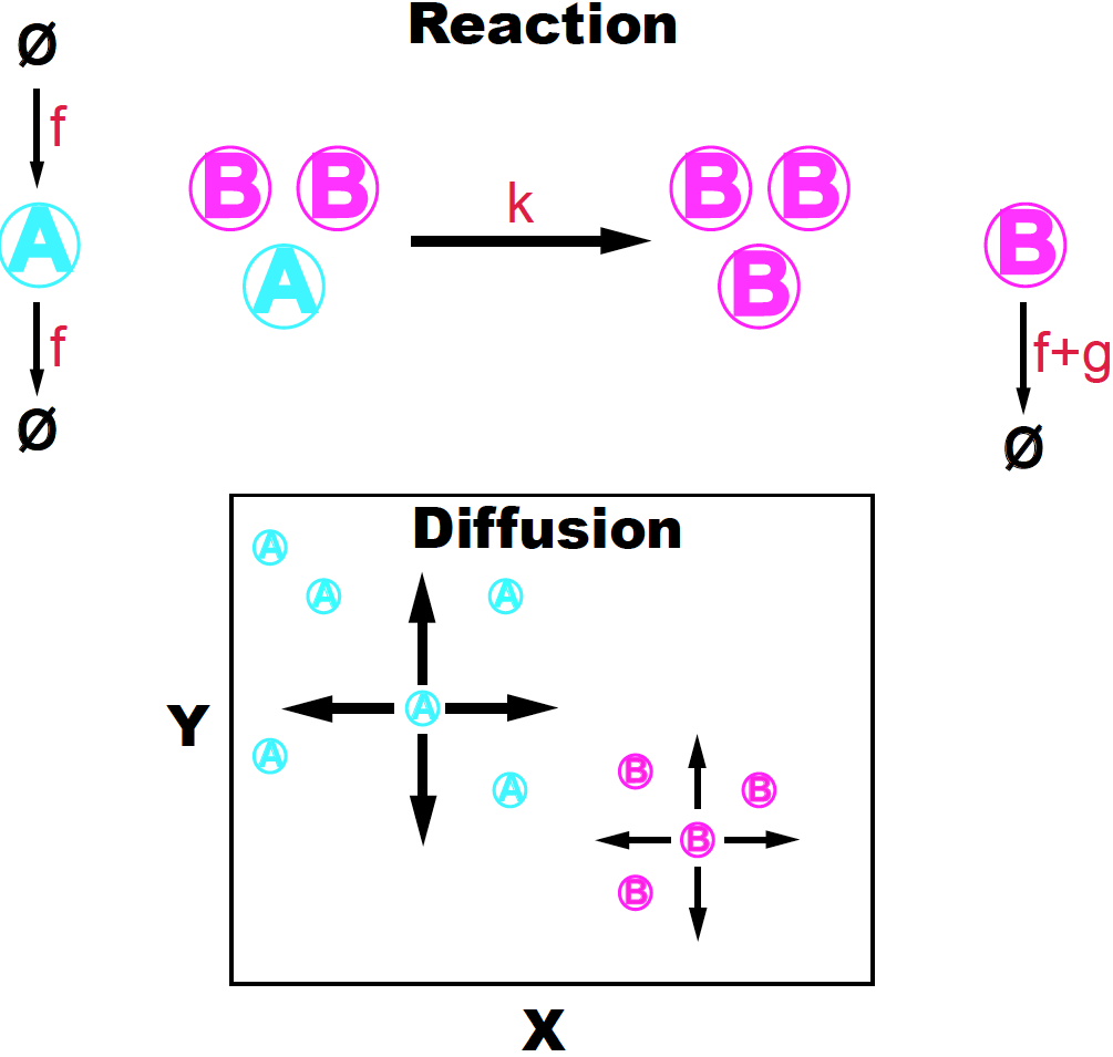
Figure 1. The Gray-Scott diffusion-reaction model. Adapted from K. Sims (http://www.karlsims.com/rd.html).
The \(A\) molecules are produced and destroyed with the same rate constant (\(f\)), that is,
\[\emptyset \overset{f}{\longrightarrow} A \overset{f}{\longrightarrow} \emptyset.\]While \(B\) can only be produced by the above reactions involving 2 \(B\)s and one \(A\), \(B\) decays on its own with a rate (\(f+g\)) larger than the one controlling the decay of \(A\).
\[B \overset{f+g}{\longrightarrow} \emptyset.\]The \(A\) and \(B\) molecules are also subject to diffusion (in both directions \(x\) and \(y\)) with diffusion constants \(D_A\) and \(D_B\) respectively. The Gray-Scott model assumes that molecules of species \(A\) diffuse faster that those of \(B\) (\(D_A>D_B\)).
The Gray-Scott continuous differential equations
The 2D reaction equation for the Gray-Scott model are
\[\begin{aligned} \frac{\delta A(x, y, t)}{\delta t} &= D_A\ \nabla^2 A(x,y,t) - k\ A B^2 + f\ (1-A)\\ \frac{\delta B(x, y, t)}{\delta t} &= D_B\ \nabla^2 B(x,y,t) + k\ A B^2 - (f+g)\ B \end{aligned}\]We cannot solve these equations analytically, but we can do a simulation using discrete time \(\Delta t\) and distance \(\Delta x\) and \(\Delta y\) intervals.
In discrete form, using the Euler algorithm, we can write
\[\begin{aligned} A(x, y, t+\Delta t) &= A(x, y, t) + \Delta t\ \left[ D_A\ \nabla^2 A(x,y,t) - k\ A(x,y,t) B^2(x,y,t) + f - f\ A(x,y,t)\right]\\ B(x, y, t+\Delta t) &= B(x, y, t) + \Delta t\ \left[ D_B\ \nabla^2 B(x,y,t) + k\ A(x,y,t) B^2(x,y,t) - (f+g)\ B(x,y,t)\right] \end{aligned}\]What about the Laplacian term?
The Laplacian operator: discrete approximation
The laplacian operator involves the second derivative respect to the space coordinates,
\[\begin{aligned} \nabla^2 A(x, y, t) &= \frac{\delta^2 A(x,y,t)}{\delta x^2} + \frac{\delta^2 A(x,y,t)}{\delta y^2}\\ \nabla^2 B(x, y, t) &= \frac{\delta^2 B(x,y,t)}{\delta x^2} + \frac{\delta^2 B(x,y,t)}{\delta y^2} \end{aligned}\]In discrete space, we can write the derivative of a function as
\[\frac{\delta^2 A(x,y,t)}{\delta x^2} \approx \frac{ A(x+\Delta x,y,t) + A(x-\Delta x,y,t) - 2A(x,y,t)}{(\Delta x)^2}\]thus and if we assume \(\Delta x = \Delta y = 1\)
\[\nabla^2 A(x, y, t) \approx \left[A(x+1,y,t) + A(x-1,y,t) + A(x,y+1,t) + A(x,y-1,t) - 4 A(x,y,t)\right].\]Which can be re-written, introducing a \(3\times 3\) kernel matrix
\[K =\left( \begin{array}{ccc} 0 & 1 & 0\\ 1 & -4 & 1\\ 0 & 1 & 0 \end{array} \right),\]as
\[\nabla^2 A(x, y, t) \approx \sum_{i=0}^{2}\sum_{j=0}^{2} A(x+i-1,y+j-1,t)\ K(i,j).\]This is called a convolution. In the image analysis lingo, this would be referred to as “approximating the laplacian function by a \(3\times 3\) convolution”.
In image analysis, they usual use convolution kernels that smooth the derivative, which result in image reconstruction with softer edges. A typical kernel, which is the one I am using in this simulation is
\[K =\left( \begin{array}{ccc} 0.25 & 0.5 & 0.25\\ 0.5 & -3 & 0.5\\ 0.25 & 0.5 & 0.25 \end{array} \right).\]You can find functions that perform this convolution for matlab and others, yet is it just a collection of sums, so it is easy to implement from scratch.
Patterns
Now, we are ready to simulate the diffusion-reaction equations of the Gray-Scott model. At a given time \(t\), we know the concentrations of both species for all points of the square,
\[A = A(x,y,t)\\ B = B(x,y,t)\]then, we can calculate the concentrations for all points at time \(t+\Delta t\),
\[A^\prime = A(x,y,t+\Delta t)\\ B^\prime = B(x,y,t+\Delta t)\]using the equations
\[\begin{aligned} A^\prime &= A + \Delta t\ \left[ D_A\ \nabla^2 A - k\ A B^2 + f -f\ A\right]\\ B^\prime &= B + \Delta t\ \left[ D_B\ \nabla^2 B + k\ A B^2 - (f+g)\ B\right] \end{aligned}\]The parameters I have used in the simulation presented in Figure 2 are
| Parameter | Value | Description |
|---|---|---|
| \(k\) | \(1.0\) | rate of producing species \(B\) |
| \(f\) | \(0.033\) | birth (and death) rate for species \(A\) |
| \(g\) | \(0.062\) | \(g+f\) is the death rate for species \(B\) |
| \(D_A\) | \(1.0\) | diffusion coefficient for species \(A\) |
| \(D_B\) | \(0.2\) | diffusion coefficient for species \(B\) |
| \(T\) | \(3000\) | total time sampled |
| \(\Delta t\) | \(1\) | time increment |
| \(L\) | \(100\) | total distance sampled in each direction |
| \(\Delta x\) | \(1\) | space increment (both in x and y directions) |
We assume that we have a lattice with \(100\times 100\) points. At each point \((x,y)\) and at each time \(t\), there is one concentration for each species \(A(x,y,t)\) and \(B(x,y,t)\).
The initial conditions (Figure 2 at \(t=0\)) correspond to having \(A=1\) everywhere in the square (in blue), and \(B=0\) everywhere in the square expect for four small (magenta) areas in which \(B=1\). Using these parameters, I obtained the patterns in Figure 2.
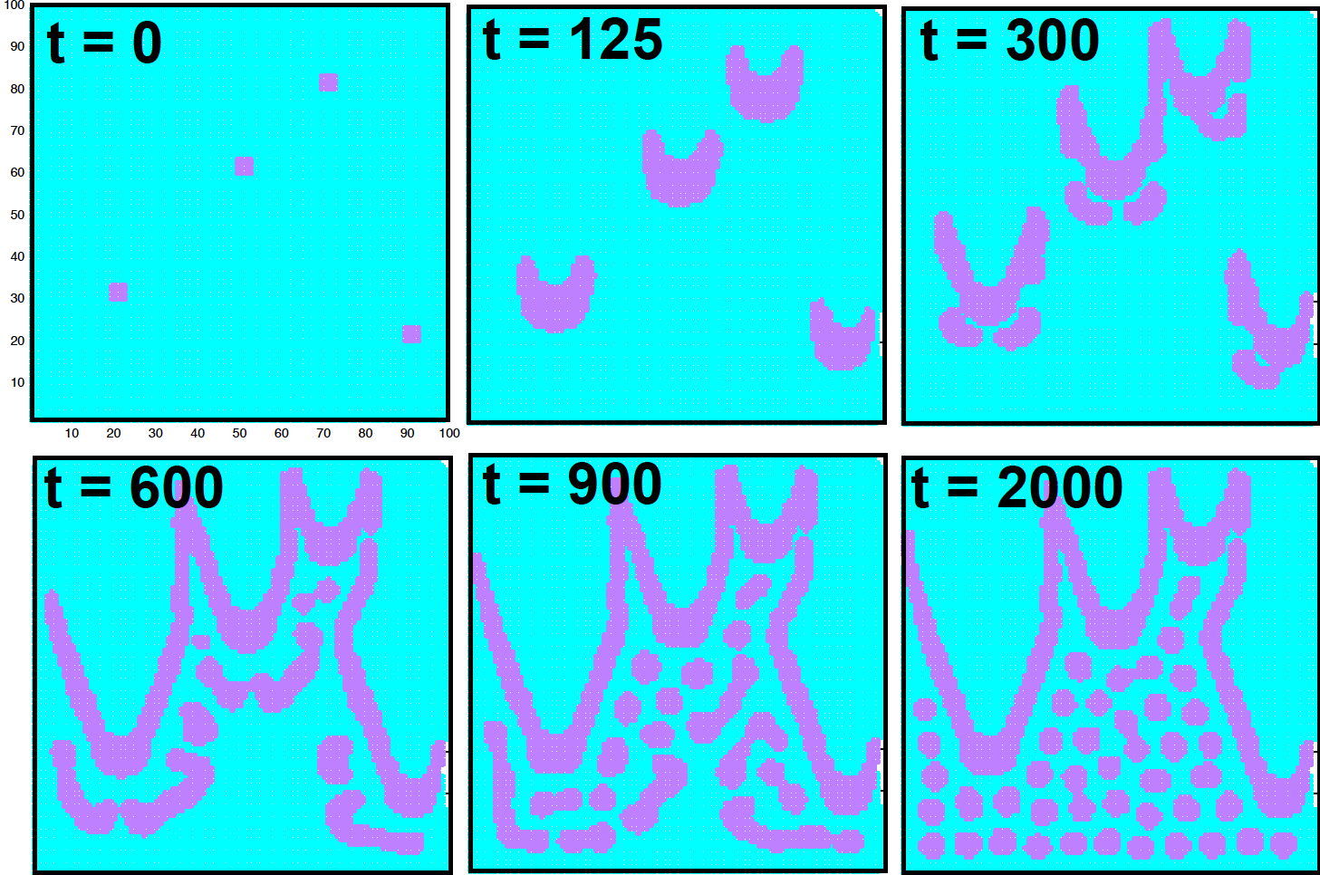
Figure 2. Patterns generated with the Gray-Scott diffusion-reaction model as a function of time, using the parameters provided in the text. We depict A molecules in cyan, and B molecules in magenta.
My images (Figure 2) are not as beautiful as Karl Sims’s are, but definitely patterns have emerged! Changing the values of the parameters, you can obtain many different patterns.
There are ways of making the pattern more complicated:
- Make diffusion occur with different constant in different directions.
- Change some the birth/death parameters as a function of the position in the plane.
- Speed up or down the reaction rate.
Biological Validation
Turing’s work was purely theoretical. You may want to check out this work by Fraden & Epstein at Brandais University, “Turing theory of morphogenesis validated”, where they observed experimentally all patterns that Turing predicted, plus seven new ones! here is the actual paper
Turing instability for a two-component system
Consider a general reaction with two components \(A\) and \(B\), as in the case of the Gray-Scott model. Let’s consider which are the conditions under which a stable set of reactions between \(A\) and \(B\), if subject to diffusion would become instable and form patterns. This phenomenon is referred to as a Turing bifurcation or Turing instability.
The diffusion-reaction system has the general form
\[\begin{aligned} \frac{\delta A(x, y, t)}{\delta t} &= D_A\ \nabla^2 A(x,y,t) + F_A(A,B)\\ \frac{\delta B(x, y, t)}{\delta t} &= D_B\ \nabla^2 B(x,y,t) + F_B(A,B) \end{aligned}\]Now consider a steady-state solution \(A_0(x,y,t)\) and \(B_0(x,y,t)\) of the reaction-only system
\[\begin{aligned} \frac{\delta A(x, y, t)}{\delta t} &= F_A(A,B)\\ \frac{\delta B(x, y, t)}{\delta t} &= F_B(A,B) \end{aligned}\]that is, the steady-state solution is characterized by
\[\begin{aligned} F_A(A^\ast,B^\ast) = 0\\ F_B(A^\ast,B^\ast) = 0 \end{aligned}\]this solution \((A^\ast, B^\ast)\) is stable if the Jacobian matrix \(J\) defined by
\[J = \left( \begin{array}{cc} \left.\frac{\delta F_A}{\delta A}\right|_\ast & \left.\frac{\delta F_A}{\delta B}\right|_\ast\\ \left.\frac{\delta F_B}{\delta A}\right|_\ast & \left.\frac{\delta F_B}{\delta B}\right|_\ast \end{array} \right) \equiv \left( \begin{array}{cc} F^\ast_{AA}&F^\ast_{AB} \\ F^\ast_{BA}&F^\ast_{BB} \end{array} \right)\]is such that the real part of the eigenvalues is negative.
For a \(2\times 2\) matrix, that is equivalent to the two conditions
- The trace in negative
- And the determinant is positive
Remember that we want to find steady solutions of the reaction that become unstable due to the diffusion process. Instability of the diffusion-reaction process for a 2-component system requires two additional conditions involving the diffusion coefficients
*
\[D_B F^\ast_{AA} + D_A F^\ast_{BB} > 0\]*
\[D_B F^\ast_{AA} + D_A F^\ast_{BB} > 2 \sqrt{D_A D_B (F^\ast_{AA} F^\ast_{BB} - F^\ast_{AB} F^\ast_{BA})}\]Derivation of these results can be found in this tutorial “Notes on turing instability and chemical instabilities” by Michael Cross (page 6), which I reproduce below.
Derivation of conditions for Turing instability for two reacting-diffusing chemicals
Turner’s discovery was that a spatially uniform and stable state (in the absence of diffusion) can become unstable due to non uniformities appearing as a result of diffusion, and patterns start to appear.
When will a diffusion-reaction start producing patterns?
For two reactants \(A\) and \(B\), subject to a reaction-diffusion process, their concentrations depending on time and space \(A(x,y,t)\) and \(B(x,y,t)\) satisfy some equations
\[\begin{aligned} \frac{\delta A(x, y, t)}{\delta t} &= F_A(A,B) + D_A\ \nabla^2 A(x,y,t)\\ \frac{\delta B(x, y, t)}{\delta t} &= F_B(A,B) + D_B\ \nabla^2 B(x,y,t). \end{aligned}\]We assume that we have found some stable solution of the non-diffusion process \(A^\ast\) and \(B^\ast\) which satisfy conditions
\[\begin{aligned} F_A(A^\ast,B^\ast) = 0\\ F_B(A^\ast,B^\ast) = 0. \end{aligned}\]Let’s now linearize around those stable solutions
\[\begin{aligned} F_A(A,B) \approx \left.\frac{\delta F_A}{\delta A}\right|_{\ast}\,(A-A^\ast) + \left.\frac{\delta F_A}{\delta B}\right|_{\ast}\,(B-B^\ast) \\ F_B(A,B) \approx \left.\frac{\delta F_B}{\delta A}\right|_{\ast}\,(A-A^\ast) + \left.\frac{\delta F_B}{\delta B}\right|_{\ast}\,(B-B^\ast). \end{aligned}\]Introducing,
\[\begin{aligned} F^\ast_{AA} = \left.\frac{\delta F_A}{\delta A}\right|_{\ast} & \quad\quad F^\ast_{AB} = \left.\frac{\delta F_A}{\delta B}\right|_{\ast}\\ F^\ast_{BA} = \left.\frac{\delta F_B}{\delta A}\right|_{\ast} & \quad\quad F^\ast_{BB} = \left.\frac{\delta F_B}{\delta B}\right|_{\ast}\\ \end{aligned}\]we can write,
\[\begin{aligned} \frac{\delta A(x, y, t)}{\delta t} &= F^\ast_{AA}\ (A-A^\ast) + F^\ast_{AB}\ (B-B^\ast) + D_A\ \nabla^2 A(x,y,t)\\ \frac{\delta B(x, y, t)}{\delta t} &= F^\ast_{BA}\ (A-A^\ast) + F^\ast_{BB}\ (B-B^\ast) + D_B\ \nabla^2 B(x,y,t). \end{aligned}\]Introducing
\[\begin{aligned} a(x,y,t) = A(x,y,t) - A^\ast\\ b(x,y,t) = B(x,y,t) - B^\ast, \end{aligned}\]we have the linearized equations
\[\begin{aligned} \frac{\delta a(x, y, t)}{\delta t} &= F^\ast_{AA}\ a(x,y,t) + F^\ast_{AB}\ b(x,y,t) + D_A\ \nabla^2 a(x,y,t)\\ \frac{\delta b(x, y, t)}{\delta t} &= F^\ast_{BA}\ a(x,y,t) + F^\ast_{BB}\ b(x,y,t) + D_B\ \nabla^2 b(x,y,t). \end{aligned}\]Introducing vectorial notation
\[\begin{aligned} \left( \begin{array}{c} \frac{\delta a}{\delta t} \\ \frac{\delta b}{\delta t} \end{array} \right) = \left( \begin{array}{cc} F^\ast_{AA} & F^\ast_{AB}\\ F^\ast_{BA} & F^\ast_{BB} \end{array} \right) \left( \begin{array}{c} a \\ b \end{array} \right) + \left( \begin{array}{cc} D_A & 0\\ 0 & D_B \end{array} \right) \left( \begin{array}{c} \nabla^2 a \\ \nabla^2 b \end{array} \right) \end{aligned}\]and
\[\begin{aligned} \mathbf{u} = \left( \begin{array}{c} a \\ b \end{array} \right) \end{aligned}\]we have the linearized equations in vectorial form,
\[\begin{aligned} \frac{\delta \mathbf{u}}{\delta t} = \left( \begin{array}{cc} F^\ast_{AA} & F^\ast_{AB}\\ F^\ast_{BA} & F^\ast_{BB} \end{array} \right) \mathbf{u} + \left( \begin{array}{cc} D_A & 0\\ 0 & D_B \end{array} \right) \nabla^2 \mathbf{u}. \end{aligned}\]We can make an ansatz that \(\mathbf{u}(x,y,t)\) has a constant term \(\mathbf{u_0}\), and such that the dependencies in time and space are given by
\[\mathbf{u}(x,y,t) = \mathbf{u_0}\ e^{\alpha\ t} e^{i\beta\ (x+y)} = \left( \begin{array}{c} a_0\ e^{\alpha\ t} e^{i\beta\ (x+y)}\\ b_0\ e^{\alpha\ t} e^{i\beta\ (x+y)} \end{array} \right),\]for some positive constants \(\alpha\) and \(\beta\).
Notice that we are assuming that both reactants \(A\) and \(B\) have the same dependencies in time and space. This is an important simplification for the results that we will find.
Under these assumptions for \(\mathbf{u}(x,y,t)\), the linear differential equation becomes
\[\begin{aligned} \alpha\ \mathbf{u} = \left( \begin{array}{cc} F^\ast_{AA} & F^\ast_{AB}\\ F^\ast_{BA} & F^\ast_{BB} \end{array} \right) \mathbf{u} - \beta^2 \left( \begin{array}{cc} D_A & 0\\ 0 & D_B \end{array} \right) \mathbf{u}. \end{aligned}\]or
\[\begin{aligned} \left( \begin{array}{cc} F^\ast_{AA}-\beta^2 D_A & F^\ast_{AB}\\ F^\ast_{BA} & F^\ast_{BB}-\beta^2 D_B \end{array} \right) \mathbf{u} = \alpha\ \mathbf{u}. \end{aligned}\]And since this results has to be true for all values of \(t\) and \(x,y\), we have
\[\begin{aligned} \left( \begin{array}{cc} F^\ast_{AA}-\beta^2 D_A & F^\ast_{AB}\\ F^\ast_{BA} & F^\ast_{BB}-\beta^2 D_B \end{array} \right) \mathbf{u_0} = \alpha\ \mathbf{u_0}. \end{aligned}\]This has now become a 2D eigenvalue problem for the 2D matrix
\[M = \left( \begin{array}{cc} F^\ast_{AA}-\beta^2 D_A & F^\ast_{AB}\\ F^\ast_{BA} & F^\ast_{BB}-\beta^2 D_B \end{array} \right).\]\(\mathbf{u_0}\) has two solutions, which are the two eigenvectors of \(M\) corresponding to its two eigenvalues
\[\alpha_{1,2} = \frac{Tr(M) \pm \sqrt{Tr^{2}(M) - 4 \det(M)}}{2},\]where the trace of \(M\) is
\[Tr(M) = F^\ast_{AA} + F^\ast_{BB} - \beta^2\ (D_A+D_B),\]and the determinant of \(M\) is given by
\[det(M) = (F^\ast_{AA} - \beta^2 D_A)\ (F^\ast_{BB} - \beta^2 D_B) - F^\ast_{AB}\ F^\ast_{BA}.\]The eigen values \(\alpha_{1,2}\) are the two solutions to the quadratic equation in \(\alpha\) resulting from imposing the condition
\[det(M-\alpha I) = det \left( \begin{array}{cc} F^\ast_{AA}-\beta^2 D_A - \alpha & F^\ast_{AB} \\ F^\ast_{BA} & F^\ast_{BB}-\beta^2 D_B-\alpha \end{array} \right) = 0.\]For a solution to be stable we need two conditions
-
(a) The solution is real, which requires \(det(M) > 0\)
-
(b) The solution is negative, which requires \(Tr(M) < 0\).
Remember that the Turing instability occurs when
-
(1) There is a stable solution in the absence of diffusion.
-
(2) The solution becomes instable when diffusion is added.
That is
-
(1) In the absence of diffusion, we have \(M_0 = M(\beta=0)\), such that
\[Tr(M_0) = F^\ast_{AA} + F^\ast_{BB},\]and
\[det(M_0) = F^\ast_{AA}\ F^\ast_{BB} - F^\ast_{AB}\ F^\ast_{BA}.\]And stability requires
* (a) $$F^\ast_{AA} + F^\ast_{BB} < 0$$ * (b) $$F^\ast_{AA}\ F^\ast_{BB} - F^\ast_{AB}\ F^\ast_{BA} >0$$ -
(2) When we add diffusion, we want the stability condition to break.
The modified trace is
\[Tr(M) = Tr(M_0) - \beta^2 (D_A+D_B),\]so \(Tr(M)\) is negative as long as \(T(M_0)\) is negative.
While \(det(M_0) > 0\), diffusion has to be capable of achieving the condition \(det(M) < 0\) in order to produce instability.
Notice that
\[det(M) = det(M_0) -\beta^2\ (D_B F^\ast_{AA} + D_A F^\ast_{BB}) + \beta^4\ D_A D_B.\]The \(det(M)\) is a parabola as a function of \(\beta^2\), and it is positive for \(\beta = 0\).
The instability condition will be achieved if the minimum of the parabola is negative.
The minimum of the parabola corresponds to
\[\beta^2_{min} = \frac{D_B F^\ast_{AA} + D_A F^\ast_{BB}}{2 D_A D_B},\]and the value of \(det(M)\) at the minimum is
\[det(M)_{min} = det(M_0) -\frac{(D_B F^\ast_{AA} + D_A F^\ast_{BB})^2}{4 D_A D_B}.\]The \(det(M)\) being negative at the bottom of the parabola then requires
- \(\beta^2_{min} > 0\) or
$$ D_B F^\ast_{AA} + D_A F^\ast_{BB} > 0. $$-
\(det(M)_{min} < 0\) or
\[det(M_0) < \frac{(D_B F^\ast_{AA} + D_A F^\ast_{BB})^2}{4 D_A D_B},\]which can be re-written as
\[4 D_A D_B (F^\ast_{AA} F^\ast_{BB} - F^\ast_{AB} F^\ast_{BA}) < (D_B F^\ast_{AA} + D_A F^\ast_{BB})^2,\]or
$$ 2 \sqrt{D_A D_B (F^\ast_{AA} F^\ast_{BB} - F^\ast_{AB} F^\ast_{BA})} < D_B F^\ast_{AA} + D_A F^\ast_{BB}. $$
Thus, we have justified the four conditions we stated without proof in the previous section.
Epilogue
Taking a quote from Turing’s paper on morphogenesis, and transferring it to our situation,
“It must be admitted that the biological examples which it has been possible to give in the present [course] are very limited. This can be ascribed quite simply to the fact that biological phenomena are usually very complicated. Taking this in combination with the relatively elementary mathematics used in this [course] one could hardly expect to find that many observed biological phenomena would be covered. [I hope], however, that the imaginary biological systems which have been treated, and the principles which have been discussed, should be of some help in interpreting real biological forms.”
This could directly apply to this course. With the difference that Turing’s “elementary mathematics” are much further advanced than mine.