MCB111: Mathematics in Biology (Fall 2024)
week 03:
Model Comparison and Hypothesis Testing
For this week’s lectures, I am following Mackay’s book, Chapter 37, and Chapter 28, in that order. MacKay’s video Lecture 10 is also relevant.
Hypothesis testing: an example
Continuing with our malaria vaccine example. Now we want to compare to a control treatment with no active ingredients. We have 40 volunteers, 30 of which receive the vaccine (V) and the other 10 receive the control (C). Of the 30 that receive the vaccine, one contracts malaria, of the 10 that receive the control treatment, three contract malaria.
Is our vaccine treatment V better than the control treatment C?
Let us assume that the probability of contracting malaria after taking the vaccine is \(f_v\), and the probability of contracting malaria under the control treatment is \(f_c\). These are the two unknown quantities, we would like to infer. What does the data tells us about them?
You may want to compare these two alternative hypotheses:
-
\(H_1\): The vaccine treatment is more effective than the control, \(f_v < f_c\).
-
\(H_0\): Both treatments have the same effectiveness, \(f_v= f_c\).
The data measurements are
\(N_v=30\) the number of subjects that took the vaccine,
\(N^+_v=1\) the number of subjects that took the vaccine and contracted malaria,
\(N_c=10\) the number of subjects in the control,
\(N^+_c=3\) the number of subjects that contracted malaria under the control treatment.
The classical test: \(\chi\)-squared test
A well used classical statistical hypothesis test is the \(\chi^2\) test.
In the \(\chi^2\) test, one compares the observed values (\(O_i\)) to the expected values (\(E_i\)) under the null hypothesis as
\[\chi^2 = \sum_{i=1}^N \frac{(O_i-E_i)^2}{E_i}.\]Then we assume that this quantity \(\chi^2\) follows the \(\chi^2\) distribution with \(n\) degrees of freedom, where \(n\) is equal to the number of measurements \(N\) minus the number of “constraint”.
In this example, the null model is that both treatment are equally effective. The probability of contracting malaria under the null hypothesis is an unknown parameter that a frequentist would estimate as
\[f_{H_0} = \frac{1+3}{30+10} = \frac{1}{10}.\]| Observed | Expected | |
|---|---|---|
| took vaccine & malaria | 1 | \(30\times \frac{1}{10} = 3\) |
| took vaccine & no malaria | 29 | \(30\times \frac{9}{10} = 27\) |
| no vaccine & malaria | 3 | \(10\times \frac{1}{10} = 1\) |
| no vaccine & no malaria | 7 | \(10\times \frac{9}{10} = 9\) |
Then, \(\chi^2\) is
\[\chi^2 = \frac{(1-3)^2}{3} + \frac{(29-27)^2}{27} + \frac{(3-1)^2}{1} + \frac{(7-9)^2}{9} = 5.926.\]To calculate the number of degrees of freedom, from the four data sets, we realize that there are two constrains (1+29=30 and 3+7 = 10), and also the fact that the \(f_{H_0}\) is not known. The result is \(4-3=1\) degrees of freedom.
A classical statistician then goes to a table for \(n=1\)-degree of freedom \(\chi^2\) values and finds
\[p = P(\chi^2 \geq 3.84) = 1 - CDF_{\chi^2_{n=1}}(3.84) = 0.05\\ p = P(\chi^2 \geq 6.64) = 1 - CDF_{\chi^2_{n=1}}(6.64) = 0.01\]and interpolating she decides that the p-value is 0.02.
What does this result mean?
-
It does not mean that there is a 98% chance that the two treatments are different.
-
It means (and this is the actual definition of a p-value) that if we were to repeat the experiment many time and the two treatments were identical, 2% of the time we will find a result with a \(\chi^2\) at least as larger than 5.926.
A lot more about p-values in the next week of lectures!
Paraphrasing Mackay: This is at best an indirect result regarding what we really want to know: have the two treatments different effectiveness?
Which \(\chi^2\) test?
The is a number of different \(\chi^2\) tests,
- Pearson’s \(\chi^2\) test, which is the one we just used above
- Yates’s test
- Cochran-Mantel-Haenszel’s test
- Tukey’s test of additivity
- portmanteau test
- …
For instance if you use Yates’s \(\chi^2\) test, which says
\[\chi^2 = \sum_{i=1}^N \frac{(\mid O_i-E_i\mid -\ 0.5)^2}{E_i},\]In classical statistics, a p-value of 0.05 is usually accepted as the boundary between rejecting (if the p-value is smaller than 0.05) or not rejecting (if p-value larger than 0.05) the null hypothesis. We would have obtained a \(\chi^2 = 3.34\). This corresponds to a p-value \(\geq 0.05\), extrapolating let’s say 0.07.
Which result would you believe?
In classical statistics, a p-value of 0.05 is usually accepted as the boundary between rejecting (if the p-value is smaller than 0.05) or not rejecting (if p-value larger than 0.05) the null hypothesis.
- Pearson’s \(\chi^2\) rejects the null hypothesis with a p-value of 0.02
- Yates’s \(\chi^2\) does not reject the null hypothesis with a p-value of 0.07
On this topic, I recommend that your read this note from David MacKay “Bayes or Chi-square? Or does it not matter?””. In this note, Mackay uses the example of inferring the language of a text by sampling random characters from the text.
Let’s now take the Bayesian approach to hypothesis testing for the vaccine question.
The Bayesian approach
As we have done before in this course, let us see what the data tells us about the possible values of the unknown parameters \(f_v\) and \(f_c\).
The posterior probability of the parameters given the data is \begin{equation} P(f_v, f_c\mid D) = \frac{P(D\mid f_v, f_c) P(f_v, f_c)}{P(D)}, \end{equation}
where the probability of the data given the parameters \(f_v\) and \(f_c\) is \begin{equation} P(D\mid f_v, f_c) = {N_v \choose N^+_v} f_v^{N^+_v} (1-f_v)^{N_v-N^+_v} {N_c \choose N^+_c} f_c^{N^+_c} (1-f_c)^{N_c-N^+_c}. \end{equation}
If we assume uniform priors \(P(f_v, f_c) = 1\), then we can factorize the posteriors and obtain \begin{equation} P(f_v, f_c\mid D) = P(f_v\mid N_v, N^+_v)P(f_c\mid N_c, N^+_c), \end{equation} and
\[\begin{aligned} P(f_v\mid N_v, N^+_v) &= \frac{f_v^{N^+_v} (1-f_v)^{N_v-N^+_v}}{\int_0^1 f ^{N^+_v} (1-f)^{N_v-N^+_v} df}, \\ P(f_c\mid N_c, N^+_c) &= \frac{f_c^{N^+_c} (1-f_c)^{N_c-N^+_c}}{\int_0^1 f ^{N^+_c} (1-f)^{N_c-N^+_c} df}. \end{aligned}\]Using the beta integral again
\[\begin{aligned} P(f_v\mid N_v, N^+_v) &= \frac{(N_v+1)!}{(N^+_v)! (N_v-N^+_v)!}\, f_v^{N^+_v} (1-f_v)^{N_v-N^+_v}, \\ P(f_c\mid N_c, N^+_c) &= \frac{(N_c+1)!}{(N^+_c)! (N_c-N^+_c)!}\, f_c^{N^+_c} (1-f_c)^{N_c-N^+_c}. \end{aligned}\]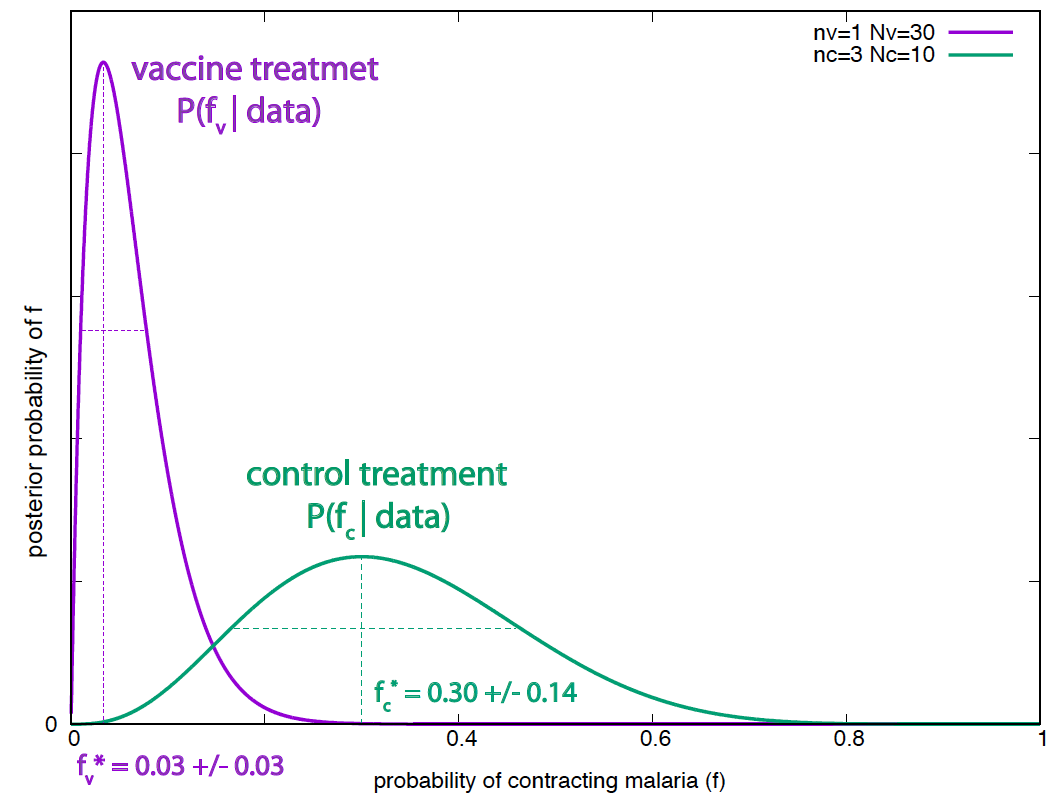
Figure 1. Posterior probabilities of the effectiveness for the vaccine and the control treatments. The parameter's standard deviation are calculated using a second order Taylor expansion around the optimal value.
For our particular example
\[\begin{aligned} P(f_v\mid N_v=30, N^+_v=1) &= \frac{31!}{1! 29!}\, f_v (1-f_v)^{29}, \\ P(f_c\mid N_c=10, N^+_c=3) &= \frac{11!}{3! 7!}\, f_c^3 (1-f_c)^{7}.\\ \end{aligned}\]The two posterior distributions are shown in Figure 1.
Exercise: reproduce on your own the optimal values and standard deviations given in Figure 1 for the parameters of the two treatments. (The standard deviations have been calculated according to the Gaussian approximation.)
The question: how probable is that \(f_v < f_c\)? has now a very clean answer
\[\begin{aligned} P(f_v<f_c\mid D) &= \int_0^1 df_c\ \int_0^{f_c} df_v\ \left[P\left(f_c\mid N_c=10, N^+_c=3\right)\times P\left(f_v\mid N_v=30, N^+_v=1\right) \right]\\ &= \int_0^1 df_c \int_0^{f_c} df_v\ \left[\frac{11!}{3! 7!} f_c^3 (1-f_c)^{7}\times \frac{31!}{1! 29!} f_v (1-f_v)^{29}\right] \end{aligned}\]This integral does not have an easy analytical expression, but it is easy to do it numerically \begin{equation} P(f_v<f_c\mid D) = 0.987. \end{equation}
This means that there is a 98.7% chance, given the data and our prior assumptions, that the vaccine treatment is more effective than the control.
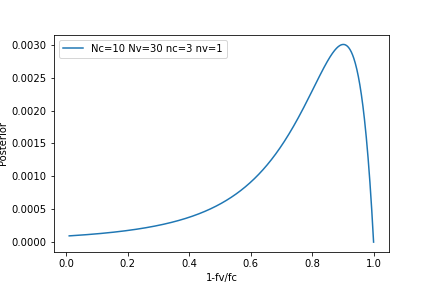
Figure 2. Vaccine effectiveness.
The question: what is the probability that \(f_v = \alpha f_c\) can be estimated using
\[\begin{aligned} P(f_v=\alpha f_c\mid D) &= \int_0^1 df_c\ \left[P\left(f_c\mid N_c=10, n_c=3\right)\times P\left(f_v=\alpha f_c\mid N_v=30, n_v=1\right) \right]\\ &= \int_0^1 df_c \left[\frac{11!}{3! 7!} f_c^{3} (1-f_c)^{7}\times \frac{31!}{1! 29!} (\alpha\ f_c) (1-\alpha\ f_c)^{29}\right] \end{aligned}\]And the vaccine effectiveness \(1-\frac{f_v}{f_c}\) is given in Figure 2.
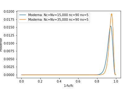
Figure 3. MODERNA mRNA vaccine effectiveness.
You can compare this result with the effectiveness obtained in Nov 2020 for the covid-19 MODERNA mRNA vaccine where 15,000 people were tested in each groups (\(N_v=N_c = 15000\)) and a total of \(95\) contracted covid-19, five of them in the vaccinated group (\(n_v=5, n_c = 90\)). The effectiveness results for that trial are given in Figure 3.
Model comparison
If we actually want to quantitatively compare the two hypotheses: \(H_1\) that \(f_v\neq f_c\) and \(H_0\) that \(f_v=f_c\), then we can use \begin{equation} \frac{P(H_1\mid D)}{P(H_0\mid D)} = \frac{P(D\mid H_1) P(H_1)}{P(D\mid H_0) P(H_0)}. \end{equation}
Giving both hypotheses equal prior probability gives \begin{equation} \frac{P(H_1\mid D)}{P(H_0\mid D)} = \frac{P(D\mid H_1)}{P(D\mid H_0)}. \end{equation}
The probability of the data under \(H_1\) (the evidence of the data under \(H_1\)) is, using marginalization, given by
\begin{equation} P(D\mid H_1) = \int_{f_v=0}^1\int_{f_c=0}^1 P(D\mid f_v, f_c, H_1) P(f_v,f_c\mid H_1)\, df_c df_v, \end{equation}
and the probability of the data under \(H_0\) is given by
\begin{equation} P(D\mid H_0) = \int_{f_v=f_c=f} P(D\mid f, f, H_0) P(f\mid H_0)\, df. \end{equation}
If we use uniform priors again, in this case for \(P(f_v,f_c\mid H_1)=1\) and \(P(f\mid H_0)=1\), then we have
\[P(D\mid H_1) = {N_c\choose N_c^+} {N_v\choose N_v^+} \int_{0}^{1} df_c\, f^{N_c^+}_c (1-f_c)^{N_c-N_c^+} \int_{0}^{1} df_v\, f^{N_v^+}_v (1-f_v)^{N_v-N_v^+},\]and
\[P(D\mid H_0) = {N_c\choose N_c^+}{N_v\choose N_v^+}\int_{0}^{1} f^{N_c^++N_v^+} (1-f)^{N_c+N_v-N^+_v-N^+_c} df.\]Then,
\[\begin{aligned} \frac{P(H_1\mid D)}{P(H_0\mid D)} &= \frac {\int_{0}^{1} f^{N_c^+}_c (1-f_c)^{N_c-N_c^+} df_c \int_{0}^{1} f^{N_v^+}_v (1-f_v)^{N_v-N_v^+} df_v } {\int_{0}^{1}df\, f^{N_c^+ + N_v^+} (1-f)^{N_c+N_v-N_c^+-N_v^+}}\\ &= \frac { \frac{(N^+_c)!(N_c-N^+_c)!}{(N_c+1)!} \frac{(N^+_v)!(N_v-N^+_v)!}{(N_v+1)!} } {\frac{(N^+_c+N^+_v)!(N_c+N_v-N^+_c-N^+_v)!}{(N_c+N_v+1)!}}\\ \end{aligned}\]In our particular example: \(N_v =30\), \(N_v^+=1\), \(N_c =10\), \(N_c^+=3\), we have
\[\frac{P(H_1\mid D)}{P(H_0\mid D)} = \frac{ \frac{1!29!}{31!} \frac{3!7!}{11!}} { \frac{4!36!}{41!} }.\]That is,
\begin{equation} \frac{P(H_1\mid D)}{P(H_0\mid D)} = \frac{0.0029}{0.00096} = 3.042. \end{equation}
This results tells us that hypothesis \(H_1\) (the vaccine treatment is more effective than the control) is 3 times more likely than the control treatment.
The raw data sort of told us that the malaria treatment was more effective. Bayesian analysis gives us a quantification of that intuitive assessment.
Consider now this other case in which the amount of data is small,
| Treatment | Vaccine | Control |
|---|---|---|
| Got malaria | 0 | 1 |
| Did not | 3 | 1 |
| Total treated | 3 | 2 |
In this case, using the expression we just deduced
\[\begin{aligned} \frac{P(H_1\mid D)}{P(H_0\mid D)} &= \frac{\int_{0}^{1} df_c\,f_c (1-f_c)\,\int_{0}^{1}df_v\,(1-f_v)^{3}}{ \int_{0}^{1}df\,f\,(1-f)^{4}}\\ &= \frac{ \frac{1!1!}{3!} \frac{0!3!}{4!}}{\frac{1!4!}{6!}}\\ &= \frac{\frac{1}{6}\frac{1}{4}}{\frac{1}{30}}\\ &= \frac{1/24}{1/30} = \frac{0.55}{0.44}. \\ \end{aligned}\]So, from our prior assumption that the two hypotheses were 50:50, the data shifts the posterior probability to 55:44 in favor of \(H_1\).
Bayesian analysis gives us a quantification of the intuitive acknowledgment that such small sample give us ``some’’ weak evidence in favor of the vaccine treatment.
Occam’s razor
Or why more complicated models can turn out to be less probable
Occam’s razor advises that if several explanations are compatible with a set of observations, one should go with the simplest. Applied to our model selection problem, Occam’s razor advised that if two different models can explain the data, we should use the one with the fewer number of parameters.
Why shall we follow Occam’s razor?
There is an aesthetic reason: more complexity is uglier, simpler is prettier. Bayesian inference offers another justification.
The plausibility of two alternative hypotheses \(H_1\) and \(H_2\) can be expressed as
\begin{equation} \frac{P(H_1\mid D)}{P(H_2\mid D)} = \frac{P(D\mid H_1) P(H_1)}{P(D\mid H_2) P(H_2)}. \end{equation}
If we use uniform priors \(P(H_1) = P(H_2)\), then the ratio of the two hypotheses is the ratio of the evidence of the data under the two hypotheses
\begin{equation} \frac{P(H_1\mid D)}{P(H_2\mid D)} = \frac{P(D\mid H_1)}{P(D\mid H_2)}. \end{equation}
Assume that \(H_1\) depends on parameter(s) \(p_1\), and \(H_2\) on parameter(s) \(p_2\). We can write,
\begin{equation} P(D\mid H_1) = \int_{p_1} P(D\mid p_1, H_1) P(p_1\mid H_1) dp_1, \end{equation}
and similarly for \(H_2\).
Remember that in many cases we have considered, the posterior probability of the parameter has a strong peak at the most probable value \(p^\ast\). We can expand the probability \(P(D\mid p_1, H_1)\) around the most probable value, defined by, \begin{equation} \frac{d}{dp_1} \left. \log P(D\mid p_1, H_1)\right|_{p_1=p_1^\ast} = 0. \end{equation}
A Taylor expansion gives us
\[\begin{equation} \log P(D\mid p_1, H_1) = \log P(D\mid p^\ast_1, H_1) - \frac{(p_1-p_1^\ast)^2}{2{\sigma_{1}^{\ast}}^2} + {\cal O}(p_1-p_1^\ast)^3, \end{equation}\]such that
\[\begin{equation} \frac{1}{\sigma_{1}^{\ast}{^2}} \equiv - \left. \frac{d^2\log P(D\mid p_1, H_1)}{dp_1^2}\right|_{p_1=p_1^\ast}. \end{equation}\]Then we can approximate \(P(D\mid p_1, H_1)\) as
\begin{equation} P(D\mid p_1, H_1) \approx P(D\mid p^\ast_1, H_1)\, e^{-\frac{(p_1-p_1^\ast)^2}{2{\sigma_1^{\ast}}^2}}. \end{equation}
This expansion goes by the name of Laplace’s Method.
Using the Laplace approximation in \(P(D\mid H_1)\), we have
\[\begin{aligned} P(D\mid H_1) &\approx P(D\mid p^\ast_1, H_1) \int_{p_1} e^{-\frac{(p_1-p_1^\ast)^2}{2{\sigma_1^{\ast}}^2}} P(p_1\mid H_1)\, dp_1. \end{aligned}\]If we assume that an uniform prior
\[\begin{equation} P(p_1\mid H_1) = \left\{ \begin{array}{ll} \frac{1}{p_1^{+} - p_1^{-}} \equiv \frac{1}{\sigma_1} & p_1^{-} \leq p \leq p_1^{+}\\ 0 & \mbox{otherwise} \end{array} \right. \end{equation}\]such that \(p_1^{-} \leq p^\ast \leq p_1^{+}\), and such that the bounds \(p^{\pm}\) are large enough
\[\begin{aligned} P(D\mid H_1) &\approx P(D\mid p^\ast_1, H_1) \int^{p_1^{+}}_{p_1^{-}}\, e^{-\frac{(p_1-p_1^\ast)^2}{2{\sigma_1^{\ast}}^2}} dp_1 \times \frac{1}{\sigma_1}\\ &\approx P(D\mid p^\ast_1, H_1)\, \sqrt{2\pi}\sigma_1^\ast \frac{1}{\sigma_1}. \\ \end{aligned}\]Then the probability ratio between the two hypotheses results to be
\[\begin{aligned} \frac{P(H_1\mid D)}{P(H_2\mid D)} &\approx \frac{ P(D\mid p^\ast_1, H_1)}{ P(D\mid p^\ast_2, H_2)}\,\times\,\frac{\sigma_1^{\ast}/\sigma_1}{\sigma_2^{\ast}/\sigma_2}\\ &\approx \mbox{best data fit}\quad\times\quad\mbox{Occam factor} \end{aligned}\]The ratio of the probability of the two hypotheses has two terms:
-
Best data fit.
This term gives us the best fit of the model to the data. If we are not Bayesian, this would be the only term to consider.
If \(H_1\) and \(H_2\) are two nested hypothesis such that \(H_2\) has more parameters and includes \(H_1\) as a particular case (\(H_1 \subset H_2\)), then it is always going to be possible for \(H_2\) to fit the data better than \(H_1\). The model with more parameters can use the extra parameters to over-fit to the data.
That is, for nested hypotheses \(H_1 \subset H_2\),
\[P(D\mid p^\ast_2, H_2) \geq P(D\mid p^\ast_1, H_1).\]This term alone would tells us that a model with more parameters would always have higher probability.
-
Bayesian Occam razor.
But we are Bayesians, then we have another term. This term is equal to the posterior accessible volume of the parameters of the hypothesis. The more posterior uncertainty we have about the model, the more it is favored.
For the two nested hypotheses \(H_1 \subset H_2\)
-
On the one hand, \begin{equation} P(D\mid p^\ast_2, H_2)\geq P(D\mid p^\ast_1, H_1) \end{equation} because \(H_2\) is going to fit the data at least as well as \(H_1\)
-
On the other hand, \begin{equation} \frac{\sigma_2^\ast}{\sigma_2} \leq \frac{\sigma_1^\ast}{\sigma_1} \end{equation} because for \(H_2\) the posterior of the parameter has a higher peak, thus it has a smaller spread.
Then for a model with more parameters to have a higher probability, the gain in the fit of the data (the data fit term), has to compensate the decrease in uncertainty about the parameter(s) (the Bayesian Occam’s razor term).
Occam’s razor Example
Let us go back to our example in Week 02 about the wait time for bacterial mutation. In that example, we assumed there was one type of bacteria, with one single mutational time constant \(\lambda\).
What if there was more than one species of bacteria with distinct mutational time constants? Can the data tell us if that is the case?
In order to do that, we want to compare two nested hypotheses:
-
\(H_1\): One mutation time constant \(\lambda\).
The probability for a bacterium to wait time \(t\) before mutating under \(H_1\) is \begin{equation} P(t\mid \lambda, H_1) = \frac{e^{-t/\lambda}}{Z(\lambda)}, \end{equation} where \(Z(\lambda)\) is determined by the normalization condition \begin{equation} Z(\lambda) = \int_{t_{-}}^{t_{+}} e^{-t/\lambda}\, dt. \end{equation} Where we have assumed that we observe the bacterial colony in the time interval times \([t_{-},t_{+}]\).
-
\(H_2\): Two mutation time constants \(\lambda_1, \lambda_2\).
The probability for a bacterium to wait time \(t\) before mutating under \(H_2\) is \begin{equation} P(t\mid \lambda_1,\lambda_2, H_2) \propto \eta \frac{e^{-t/\lambda_1}}{Z(\lambda_1)} + (1-\eta) \frac{e^{-t/\lambda_2}}{Z(\lambda_2)}, \end{equation}
such that there is a probability \(\eta\) that the bacterium mutates with rate \(\lambda_1\) and a probability \(1-\eta\) that it mutates with rate \(\lambda_2\). For simplicity, we assume that \(\eta\) is a fixed value.
We want to calculate the ratio of the probability of the two hypotheses, which as we have seen before is given by \begin{equation} \frac{P(H_1\mid D)}{P(H_2\mid D)} = \frac{P(D\mid H_1)}{P(D\mid H_2)}, \end{equation} assuming an equal prior for the two hypotheses.
Let’s calculate the evidences \(P(D\mid H_1)\) and \(P(D\mid H_2)\) for the two hypotheses. If we assume we have \(N\) data that correspond to mutation times \(t_1,\ldots,t_N\), then
-
Evidence for H_1: For a given parameter \(\lambda\) we have, \begin{equation} P(D\mid \lambda, H_1) = \frac{e^{-\sum_i t_i/\lambda}}{Z^N(\lambda)}. \end{equation}
The evidence is obtained by marginalization over all allowed values of \(\lambda\) as
\[\begin{aligned} P(D\mid H_1) &= \int_{\lambda} P(D\mid \lambda, H_1) P(\lambda\mid H_1)\, d\lambda\\ &= \int_{\lambda^-}^{\lambda^+} \frac{e^{-\sum_i t_i/\lambda}}{Z^N(\lambda)} \frac{1}{\lambda^{+}-\lambda^{-}}\, d\lambda\\ &= \frac{1}{\sigma}\int_{\lambda^-}^{\lambda^+} \frac{e^{-\sum_i t_i/\lambda}}{Z^N(\lambda)}\, d\lambda. \end{aligned}\]Here, I assume a uniform prior for \(\lambda\) (which can vary in \([\lambda^{-},\lambda^{+}]\)) given by
\[P(\lambda\mid H_1) = \left\{ \begin{array}{ll} \frac{1}{\lambda^{+}-\lambda^{-}} = \frac{1}{\sigma} & \lambda^{-}\leq\lambda\leq\lambda^{+}\\ 0 & \mbox{otherwise} \end{array} \right.\] -
Evidence for H_2: For two given parameters \(\lambda_1, \lambda_2\) we have,
\[\begin{aligned} P(D\mid \lambda_1, \lambda_2, H_1) &= \prod_i \left[\eta \frac{e^{-t_i/\lambda_1}}{Z(\lambda_1)} + (1-\eta) \frac{e^{-t_i/\lambda_2}}{Z(\lambda_2)}\right]\\ \end{aligned}\]The evidence is obtained by marginalization over all allowed values of \(\lambda_1\) and \(\lambda_2\) as
\[\begin{aligned} P(D\mid H_2) &= \int_{\lambda_1}\int_{\lambda_2} P(D\mid \lambda_1,\lambda_2, H_2) P(\lambda_1,\lambda_2\mid H_2)\, d\lambda_1 d\lambda_2\\ &= \int_{\lambda_1^-}^{\lambda_1^+}\int_{\lambda_2^-}^{\lambda_2^+} \prod_i \left[\eta \frac{e^{-t_i/\lambda_1}}{Z(\lambda_1)} + (1-\eta) \frac{e^{-t_i/\lambda_2}}{Z(\lambda_2)} \right] \frac{1}{\lambda_1^{+}-\lambda_1^{-}}\frac{1}{\lambda_2^{+}-\lambda_2^{-}}\, d\lambda_1 d\lambda_2\\ &= \frac{1}{\sigma_{1}\sigma_{2}}\int_{\lambda_1^-}^{\lambda_1^+}\int_{\lambda_2^-}^{\lambda_2^+} \prod_i \left[\eta \frac{e^{-t_i/\lambda_1}}{Z(\lambda_1)} + (1-\eta) \frac{e^{- t_i/\lambda_2}}{Z(\lambda_2)} \right] \end{aligned}\]Uniform priors are also assumed for \(\lambda_1\) and \(\lambda_2\) and \(\sigma_{1}\equiv \lambda^{+}_{1}-\lambda^{-}_{1}\), \(\sigma_{2}\equiv \lambda^{+}_{2}-\lambda^{-}_{2}\).
The ratio of the two evidences gives us the ratio of the two hypotheses. The integrals in the evidences can be easily calculated numerically.
For the example of Week 02, the data was \(N = 6\) \begin{equation} {t_1,\ldots,t_6}= {1.2,2.1,3.4,4.1,7,11}. \end{equation}
Assuming \(\eta = 0.5\), \(t_{-} = 1\) mins, \(t_{+} = 20\) mins; and \(\lambda^{-}= \lambda_1^{-}= \lambda_2^{-}= 0.05\), and \(\lambda^{+}= \lambda_1^{+}= \lambda_2^{+}=80\), produces,
\[\begin{aligned} P(H_1\mid \{1.2,2.1,3.4,4.1,7,11\}) &= e^{-16.213},\\ P(H_2\mid \{1.2,2.1,3.4,4.1,7,11\}) &= e^{-16.499}.\\ \end{aligned}\]That is
\begin{equation} \frac{P(H_1\mid {1.2,2.1,3.4,4.1,7,11})}{P(H_2\mid {1.2,2.1,3.4,4.1,7,11})} = e^{0.286} = 1.33. \end{equation}
That is, the amount of data is small, and the evidence favors \(H_1\) but only slightly.
Question: what would you do if you wanted to relax the condition that the mixing parameter \(\eta\) has a fixed value. Can you do inference to determine its value given the data?