MCB111: Mathematics in Biology (Fall 2024)
- One dimensional Random Walks (discrete space and time)
- Brownian Movement (continuous time and space)
week 09:
Random Walks in Biology
For these lectures, I have followed Howard Berg’s book “Random walks in biology”, as well as Chapter 7 of Philip Nelson’s book “Physical models of living systems”.
Most molecules inside a cell are subject to thermal fluctuations. Organells inside a cell are also in constant motion. Cells (such as bacterial colonies) also interact with each other in aqueous environments and are subject to constant movement. This week, we are going to describe the basic mathematical rules that control this type of thermal random movement.
One dimensional Random Walks (discrete space and time)
The concept of random walk was first introduced by Karl Pearson in 1905, and he used random walks to describe how mosquito could infests a forest. At about the same time, Albert Einstein introduced Brownian movement to describe the movement of a particle of dust in the air.
This situation is the simplest possible example of a diffusion problem. Particles start at time \(t=0\) and position \(x = 0\). Particles move according to the following rules:
Assumptions
-
Each particle moves after a fixed step time \(\tau\) a fixed step distance \(\delta\) to the left or to the right.
-
Each particle steps left or right with probabilities \(p\) and \(q=1-p\) respectively.
-
Particles move independently from each other.
-
Particles don’t get destroyed or created from other particles.
In Figure 1, I show a simulation for 10 particles for different values of the Bernoulli parameter \(p\) of stepping into the left. All particles start at time \(t=0\) in position \(x=0\).
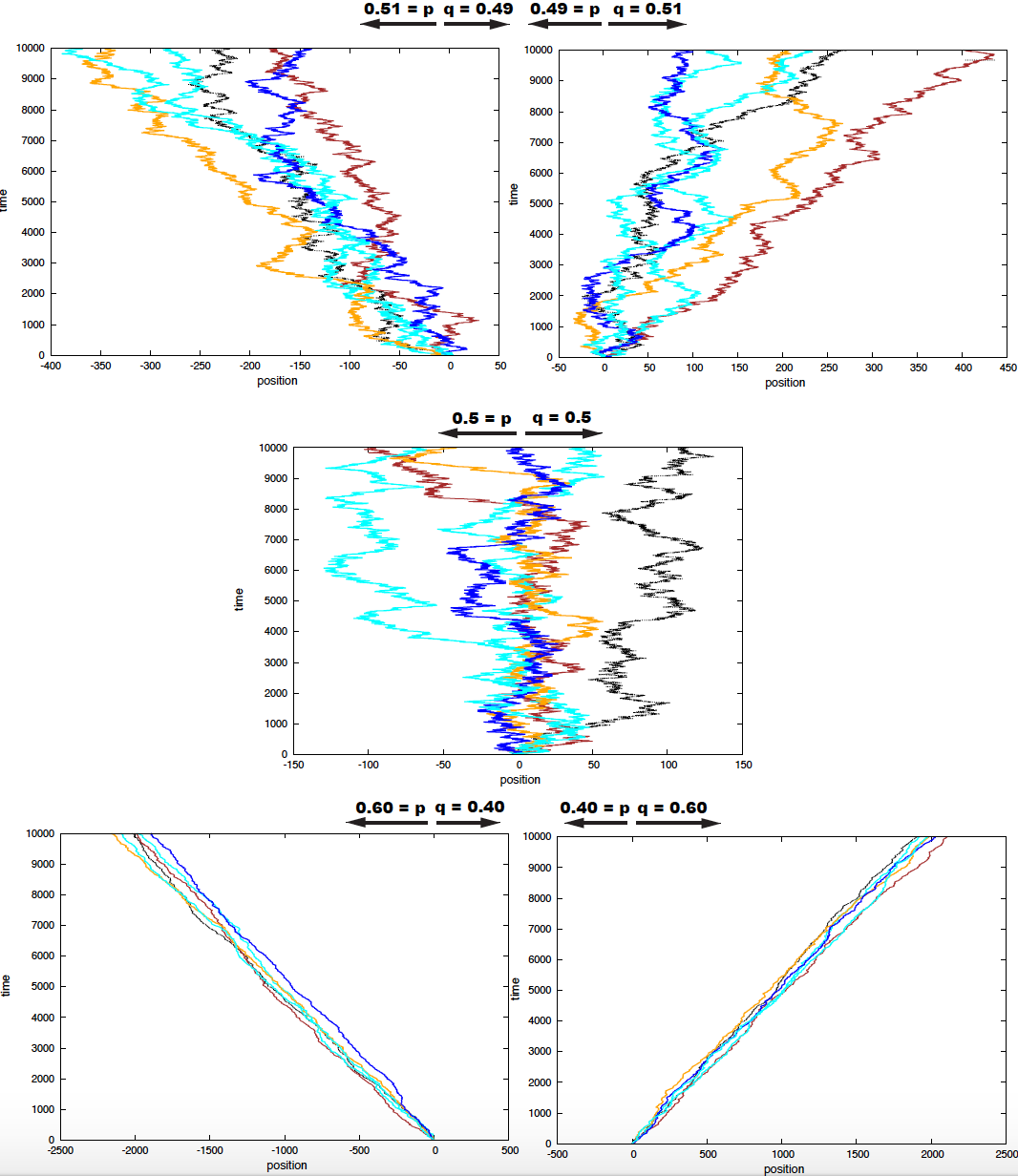
Figure 1. Five examples of 10 particles performing 1D random walks under different Bernoulli parameters.
The probability distribution
After time \(t= N\tau\) (or \(N\) steps), a given particle, will be at a position \(x=m\delta\). The probability distribution for one particle to be at position \(m\) after \(N\) steps \(P_N(m)\) follows a binomial distribution.
If we assume that the particle moved \(l\) steps to the left (and \(N-l\) steps to the right), then we have
\[P_N(l) = \frac{N!}{l! (N-l)!} p^{l}\ (1-p)^{N-l}.\]Using the relationships,
\[m = (N-l) - l = N -2l,\]or
\[l = \frac{N - m}{2}\\ N-l = \frac{N + m}{2}.\]The probability of the particle finding itself at position \(m\) (\(x = m\ \delta\)) after wandering for \(N\) steps (\(t= N\ \tau\)) is
\[\begin{aligned} P_N(m) &= \frac{N!}{l! (N-l)!} p^{l}\ (1-p)^{N-l}\\ &= \frac{N!}{\left(\frac{N-m}{2}\right)! \left(\frac{N + m}{2}\right)!} p^{\frac{N-m}{2}}\ (1-p)^{\frac{N+m}{2}} \end{aligned}\]Properties
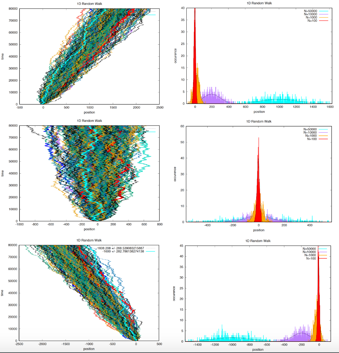
Figure 2. Three examples of 500 particles performing 1D random walks under different Bernoulli parameters. Top p= 0.4, middle p = 0.5, bottom p = 0.6. For each condition, in the right panels, we display the probability distribution for the displacement at different steps values n = 100, 1,000, 10,000, and 1000,000.
-
The mean position is proportional to the number of steps (the elapsed time)
The mean of \(P_N(m)\) can be calculated as
\[\langle m\rangle = \sum_{m} m\ P_N(m) = \sum_{l} (N - 2l)\ P_N(l) = N - 2 \sum_{l} l\ P_N(l).\]And remembering that for a binomial distribution \(\langle l \rangle = N p\), then
That is, the mean is proportional to the number of steps.
For the particular case that \(p = q = 1/2\), there is no net displacement. As we can observe for the middle graph in Figure 1. When \(p = q\), we say that the random walk has no drift.
-
The standard deviation of the displacement is proportional to the square root of the elapsed time.
The variance of \(P_N(m)\) can be calculated easily by remembering that \(m = N - 2l\), as
\[Var(m) = 4 Var(l) = 4 N p q.\]Then, the standard deviation is given by
Thus, the standard deviation grows with the square root of the elapsed time (\(N\)). We can observe such behavior in Figure 2.
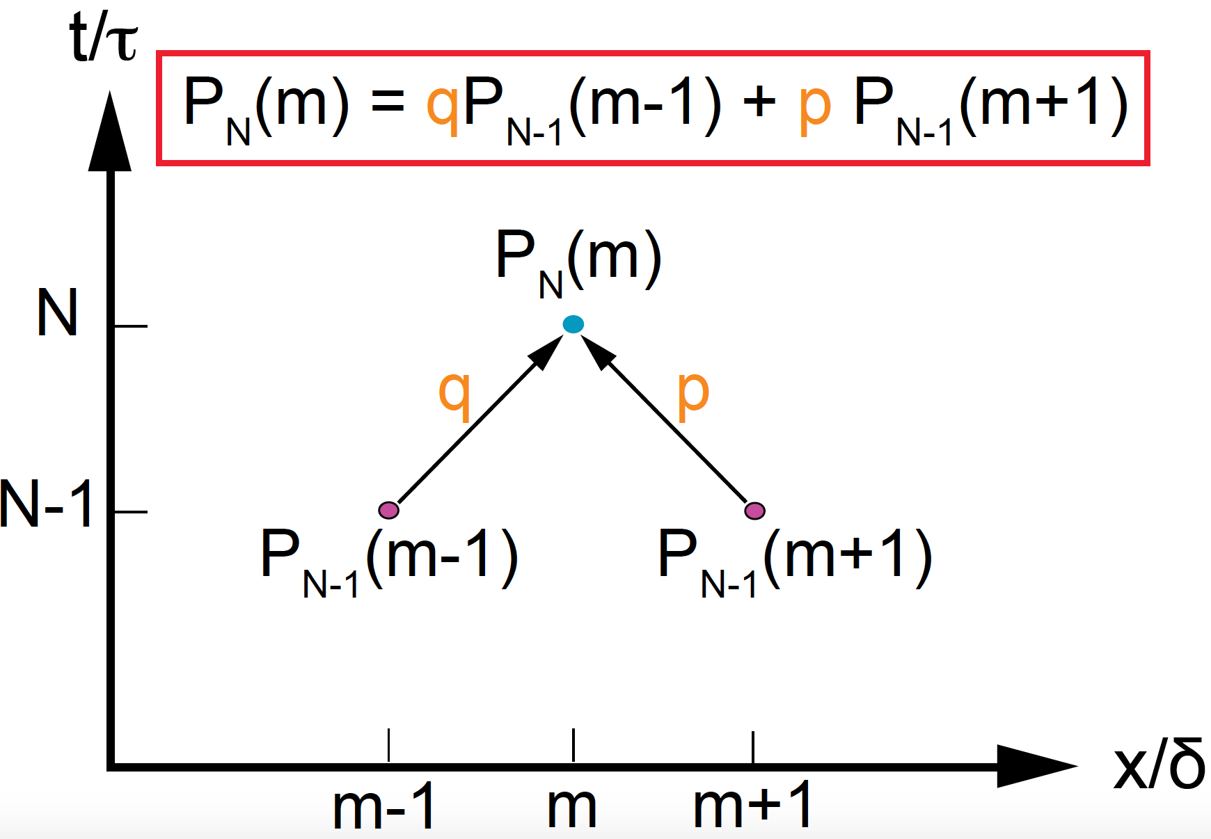
Figure 3. The difference equation satisfied by the probability of finding a particle at position m, after time N.
-
Very small particles that can take a very large number of steps per second (lysozymes in a cell is a good example). In that case, where
\[N\rightarrow \infty \quad N\ p \rightarrow \infty,\]the Binomial distribution (by the central limit theorem) approximates a Gaussian distribution, with mean \(\mu\) and standard deviation \(\sigma\) given by
\[\begin{aligned} \mu &= \langle m\rangle = N\ (p-q)\\ \sigma &= \sqrt{Var(m)} = 2 \sqrt{N p q }. \end{aligned}\]That is for \(N\) very large,
\[P_N(m\mid p) \rightarrow P(m\mid \mu, \sigma)\ dm = \frac{1}{\sqrt{2\pi \sigma^2}} e^{-(m-\mu)^2/2\sigma^2}\ dm\]Where \(P(m\mid \mu, \sigma)\) is the probability of a particle moving from m \(m\) to \(m+dm\), where \(dm\) is very small.
In Figure 2, I show several examples with a large number of trajectories, where we observe the behavior of a 1D random walk, and the fit to the Gaussian approximation.
-
The random walk has no memory. The next position depends only on where we are, not on how we got there. That is, it is a Markovian process.
The probability \(P_N(m)\) satisfies the equation (see Figure 3).
This is known as the master equation of the diffusion stochastic process.
Random walk with drunken pauses
A slight modification of the process can be achieve if we assume that \(p+q <1\) and that the system “does nothing” with probability \(z=1-p-q\). This is called a random walk with drunken pauses. The master equation with drunken pauses is given by
In this case, if \(l\) is the number of left movement, and \(n\) is the number of steps with no movement the net displacement to the right \(m\) is given by the number of moves to the right \(N-l-n\) minus the number of movements to the left \(l\),
\[m = N - (l+n) - l = N - 2l - n.\]The mean value of the displacement is given by
\[\langle m\rangle = N - 2N\ p - N\ z = N (1 - 2p -z) = N (q+z-p - z) = N(q-p)\]the same as in the case with no drunken pauses.
An the standard deviation of the displacement is given by
\[\begin{aligned} Var(m) &= 4 Var(l) + Var(n)\\ &= 4 N\ p(1-p) + N\ z (1-z)\\ &=4 N\ p(q+z) + N\ z(p+q). \end{aligned}\]The probability of capture
A random walk starts at \(x = 0\), what is the probability that it reaches a given position \(i > 0\)? (Figure 4).
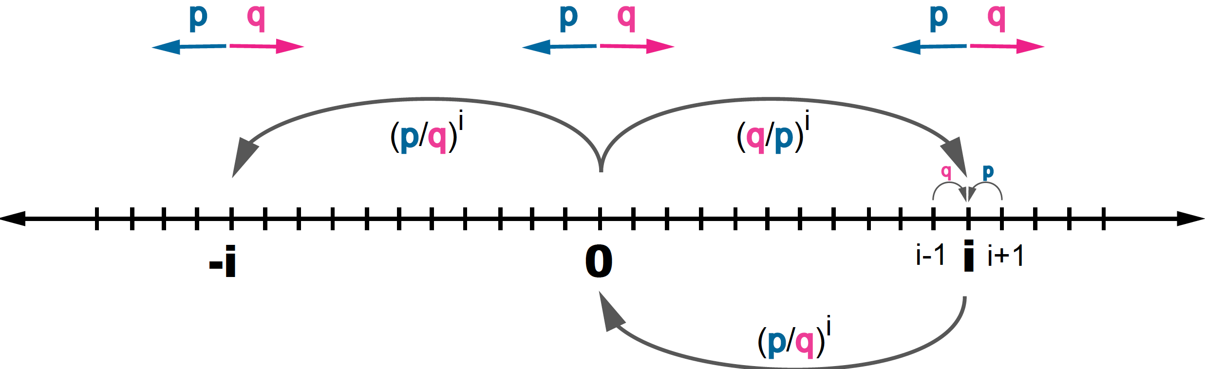
Figure 4. For a 1D random walk, probability of starting at point 0, and reaching another point i > 0.
We are going to use the Markov equation to solve this question.
Lets name such probability \(P(i\mid 0)\), for \(i > 0\). We are going to assume that the particle is in a large media, and there is, not risk of reaching the end, that is
\[\begin{aligned} P(\infty\mid 0) &= 0 \end{aligned}\]According to the Markov equation,
\[\begin{aligned} P(i\mid 0) &= P(i-1\mid 0)\ p((i-1)\rightarrow i) + P(i+1\mid 0)\ p((i+1)\rightarrow i)\\ &= P(i-1\mid 0)\ q + P(i+1\mid 0)\ p. \end{aligned}\]To find the form of \(P(i\mid 0)\), let’s make an ansatz of the solution. I propose
\[P(i\mid 0) = A \beta^{i} + C\]The no boundary condition is satisfied if
\[C = 0 \quad \mbox{and}\quad 0 < \beta \leq 1.\]Then we have
\[P(i\mid 0) = A \beta^{i}\quad \mbox{for}\quad 0 < \beta \leq 1.\]Because the particle is at position zero, trivially \(P(0\mid 0) = 1\), then \(A = 1\).
Then we have
\[P(i\mid 0) = \beta^{i}\quad \mbox{for}\quad 0 < \beta \leq 1.\]Using the Markov equation we can determine the value of \(\beta\)
\[\beta^i = \beta^{i-1} q + \beta^{i+1} p\]or multiplying by \(\beta^{-i}\)
\[1 = \frac{1}{\beta} q + \beta p,\]which can be written as the second order equation
\[p\ \beta^2 -\beta + q = 0.\]The solutions are
\[\beta = \frac{1\pm \sqrt{1-4 p q}}{2p} = \frac{1\pm \sqrt{(p-q)^2}}{2p} = \frac{1\pm (p-q)}{2p},\]resulting in
\[\begin{aligned} \beta &= 1,\\ \beta &= \frac{q}{p}, \end{aligned}\]then
\[P(i\mid 0) = \left\{ \begin{array}{ll} \left(\frac{q}{p}\right)^{i}\quad \mbox{for} & q < p\\ 1& q \geq p \end{array} \right.\]In summary:
- For \(q > p\), the particle will always reach position \(i\)
- Even for \(q < p\), there is a chance of reaching \(i\), given by \((q/p)^i\).
- In the particular case \(p = q = 0.5\) (an unbiased random walk), position \(i\) is always eventually reached.
This mathematical framework applies for problems such as
-
A very small population of individuals, where birth has probability \(q\) and death has probability \(p\). Even if there is no net growth (\(q < p\)), the population can reach a given size \(i\) with probability \((q/p)^i\).
-
A gambler with no capital, where \(q\) is the probability of winning. Even if \(q < 0.5\) there is a chance of winning \(i\) amount of money by probability \((q/p)^i\).
Reciprocally, if starting at position \(i\), the probability of reaching \(0\) is (see Figure 4)
\[P(0\mid i) = \left\{ \begin{array}{ll} \left(\frac{p}{q}\right)^{i}\quad \mbox{for} & p < q\\ 1& p \geq q \end{array} \right.\]That is,
-
A population of size \(i\), even with a net growth rate \(q > p\), there is a chance of extinction given by \((p/q)^i\).
-
A gambler with a capital \(i\), where \(q\) is the probability of winning. Even if \(q > 0.5\) there is a chance of loosing all money given by \((p/q)^i\).
Time to capture (hitting times)
Ok, so a population can grow to an arbitrary large size even if there is not net growth, but how long would that take?
The expected time it would take to go in a random walk from position \(i\) to position \(j\) is called a hitting time \(h(j\mid i)\).
Using the Markov recursion again
\[h(i\mid 0) = 1 + h(i+1\mid 0)\ p + h(i-1\mid 0)\ q.\]Using the ansatz,
\[h(i\mid 0) = A\ i\]we have
\[A\ i = 1 + A\ (i+1)\ p + A\ (i-1)\ q\]that is
\[A\ i = 1 + A\ i\ (p+q) + A\ p - A\ q\]remembering that \(p+q=1\),
\[0 = 1 - A\ (q - p)\]resulting in
\[A = \frac{1}{q-p}\]The final result for the hitting time is, for \(i > 0\),
\[h(i\mid 0) =\left\{ \begin{array}{ll} \frac{i}{q-p} & \mbox{if}\, q > p\\ \frac{i}{p-q} & \mbox{if}\, q < p \end{array} \right.\]This expression for hitting times tells us
- In general, hitting times are not symmetric.
- For an unbiased random walk (\(q=p\)), it would take infinite time to return to the origin.
- For a population of size \(i\), the time it would take to reach extinction is proportional so the size of the population.
The answer to our leading questions: how long it would take to a population to grow to a given size \(M\) when there is no positive growth, birth rate (\(q\)) < death rate (\(p\)) is:
- Time is proportional to the size \(M\).
- Time is inversely proportional to \(q-p\)
- It would take infinite time if the rates of birth and death are identical.
2D Random Walks
The assumptions of a 1D random walk can be generalized for two or three dimensions. If we further assume that the movements in the x and y directions are independent from each other, and that each movement occurs simultaneously in both directions, so the movement is always diagonal, then we can simulate a 2D random walk, as described in Figure 5.
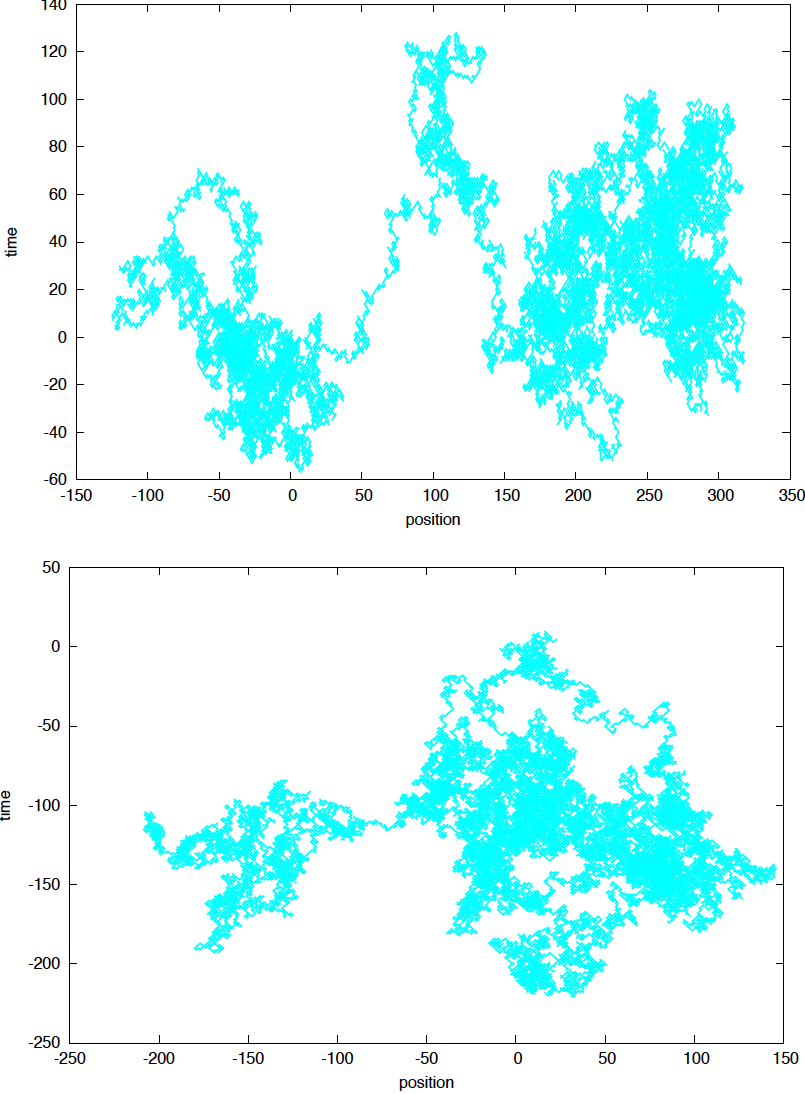
Figure 5. Sampled two dimensional random walks with N= 50,000 steps each and no drift (p=q).
In Figure 5, we observe an important property of random walks: because it takes a shorter time to explore closer regions, the particle tends to explore proximal regions, before exploring more distant regions. After one rarer event of wandering away, it process to do more local explorations. Because the random walk has no memory, there is never a knowledge of what has or has not been explored in the past.
Brownian Movement (continuous time and space)
Brownian movement is named after the botanist Robert Brown, who in 1827 observed the movement of particles trapped inside pollen grains. Brownian motion refers to the macroscopic picture that emerges from a random walk.
Lysozymes is a protein commonly found in tear, saliva, mucus, egg white, cytoplasmic compartments and other secretions. Lysozymes can destroy the cell walls of bacteria. For a lysozymes, we have the following approximate parameters
\[\begin{aligned} \delta &= \mbox{path between collisions} \approx 10^{-10} cm\\ \tau &= \mbox{time between collisions} \approx 10^{-13} sec\\ \frac{\delta}{\tau} &= \mbox{ thermal velocity} = 10^3 cm/sec. \end{aligned}\]This is a considerable speed. At that speed, the lysozyme would ran a marathon in 1.3 hours. The lysozyme takes \(N = \frac{1}{\tau} = 10^{13}\) steps per second.
When you take the continuous time and space limit, then a random walk becomes Brownian movement.
We assume no drift for the movement of lysozymes, and that the particle is at position zero at time zero.
The mean displacement of each molecule at time \(t\) is
\[\langle x(t)\rangle = 0\]And the variance (or mean-square displacement) (\(t=N\tau\) and \(x= m \delta\))
\[\begin{aligned} \langle x(t)^2\rangle &= Var(m)\ \delta^2 \\ &= 4 N p\ q\ \delta^2 \\ &= 4 \left(\frac{t}{\tau}\right) p\ q\ \delta^2 \\ &= t\ \frac{\delta^2}{\tau}. \end{aligned}\]We introduce a new variable the Diffusion coefficient
\[D \equiv \frac{1}{2}\frac{\delta^2}{\tau}.\]The diffusion coefficient characterizes how a particular type of particles wanders (migrated). It depends on properties of the particle such as size, as well as on external ones such as the structure of the media, and the temperature of the media.
Then, the variance is given by
\[\langle x(t)^2\rangle = 2 D t,\]and the mean-square deviation of the displacement is
\[\sigma = \sqrt{2Dt}.\]And using the Gaussian approximation, the probability of finding the particle at position \(x\) at time \(t\) is
This result generalizes for two and three dimensions. Movement in each direction is independent from each other, which results in
\[\langle x^2\rangle = \langle y^2\rangle = \langle z^2\rangle = 2D\ t.\]Introducing \(r^2 = x^2+y^2\) in 2D and \(r^2 = x^2+y^2+z^2\) in 3D, we have
\[P(r\mid t) = \frac{1}{(4\pi Dt)} e^{-\frac{r^2}{4Dt}} \mbox{ for 2D}\\ P(r\mid t) = \frac{1}{(4\pi Dt)^{3/2}} e^{-\frac{r^2}{4Dt}} \mbox{ for 3D}\\\]How fast is Brownian motion?
Well, it depends on how much time you have been wandering. While the mean displacement is zero, the mean squared displacement grows with time.
\[\begin{aligned} \langle x(t)\rangle &= 0\\ \langle x^2(t)\rangle &= 2D t\\ \end{aligned}\]For the lysozyme particles, the Diffusion coefficient takes the value
\[D = \frac{1}{2} \frac{\delta^2}{\tau} = 10^{-6} cm^2/sec.\]This is a standard value for small particles. Here are some examples of the \(\sigma(t) = \sqrt{\langle x^2(t)\rangle}\) obtained at different times
\[\sigma = \sqrt{2Dt}\quad \mbox{or}\quad t = \frac{\sigma^2}{2D}\]| t | \(\sqrt{\langle x^2(t)\rangle}\) | |
|---|---|---|
| 1 \(\mu\) | \(10^{-4}\) cm | size of a bacterium |
| 1 ms | \(10^{-3}\) cm | size of a neuron’s cell body |
| 8 min | 0.1 mm | length of a neuron’s dendrite |
| 6 days | 1 cm | length of a neuron’s axon |
In Brownian motion, the mean-square deviation of the displacement grows with the square-root of the time. There is not such thing as a “Diffusion velocity”.
The Diffusion Equations
The diffusion equations describe the macroscopic behavior of a random walk when both time and space are continuous variables. The diffusion equations are also referred to as Fick’s equations.
We are going to derive the diffusion equations in two different ways. We assume a random walk process in which \(p = q\).
Using the Markovian condition introduced above, we can rewrite
\[P_{N+1}(m) = \frac{1}{2} P_N(m-1) + \frac{1}{2} P_N(m+1)\]as
\[P_{N+1}(m) - P_N(m) = \frac{1}{2} \left[P_N(m-1) +P_N(m+1) - 2 P_N(m)\right]\]Introducing
\[P(x,t) = P_N(m)\quad \mbox{for}\ x= m\delta, t = N\tau,\]and remembering that
\[\frac{\delta P(x,t)}{\delta t} = \lim_{\tau\rightarrow 0} \frac{P(x,t+\tau) - P(x,t)}{\tau},\]and
\[\frac{\delta^2 P(x,t)}{\delta x^2} = \lim_{\delta\rightarrow 0} \frac{P(x-\delta,t) +P(x+\delta,t) - 2 P(x,t)}{\delta^2},\]then taking the continuous limit \(\tau,\delta\rightarrow 0\), the above equation becomes a differential equation
\[\tau\ \frac{\delta P}{\delta t} = \frac{1}{2} \delta^2 \frac{\delta^2 P}{\delta x^2}\]or
\[\frac{\delta P}{\delta t} = \frac{1}{2} \frac{\delta^2}{\tau} \frac{\delta^2 P}{\delta x^2}\]which result in the diffusion equation
\[\frac{\delta P}{\delta t} = D \frac{\delta^2 P}{\delta x^2},\]where \(D\) is the diffusion coefficient.
Let’s also look at a more intuitive derivation given by Berg in Chapter 2.
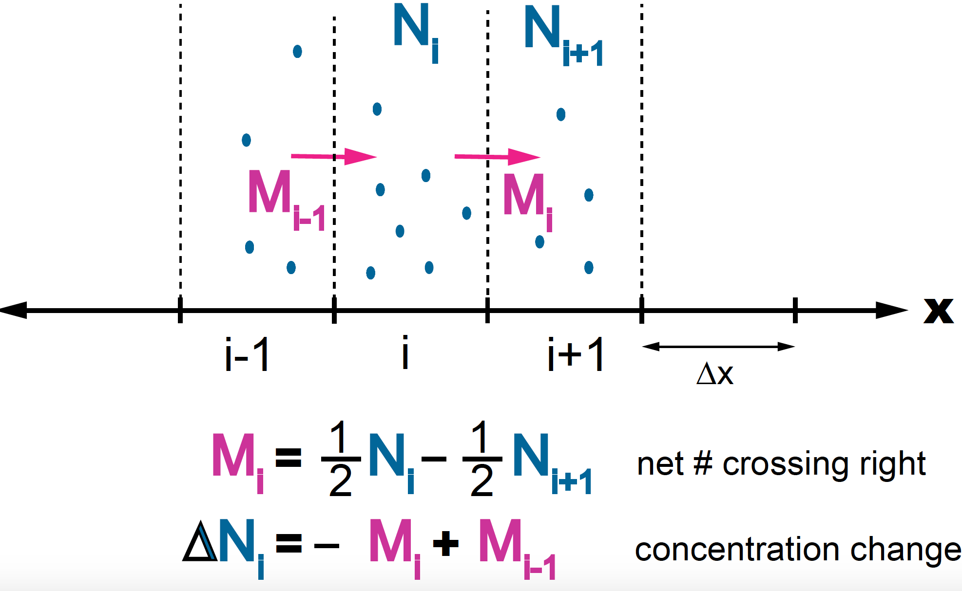
Figure 6. Diffusion for an unbiased random walk. At time t there are N(i) particles at position i and N(i+1) at position i+1. At the next step, half of the N(i) particles have move right to i+1 and half of the N(i+1) particles have moved left to i.
At time \(t\), there are \(N_i\) in between i and i+1, and \(N_{i+1}\) particles between \(i+1\) and \(i+2\). At time \(t+\tau\), there has been a flux of particles, such that half of the \(N_i\) particles have moved to \(i+1\), and half of the \(N_{i+1}\) particles have moved left to \(i\). The net flux of particles from \(i\) to \(i+1\), named \(M_i\) is given by
\[M_i = \frac{1}{2} N_{i} - \frac{1}{2} N_{i+1}.\]Equivalently, the change in the number of particles at position \(i\) between times \(t\) and \(t+\tau\) is given by the particles that left \((-M_i)\) plus the particles that arrived
\[\Delta N_i = -M_{i} + M_{i-1}.\]Let’s introduce
-
Flux, or particles crossing per unit of time at a given position \(i\)
\[J_i = \frac{M_i}{\tau}.\] -
Concentration, or particles per unit length at a given position \(i\)
\[C_i = \frac{N_i}{\delta}.\]
Then the first equation can be re-written as
\[\begin{aligned} J_i &= -\frac{1}{2\tau}(N_{i+1}-N_i)\\ &= -\frac{1}{2\tau}\ (\delta C_{i+1}-\delta C_i)\\ &= -\frac{\delta^2}{2\tau}\ \frac{C_{i+1}-C_i}{\delta}\\ &= -D\ \frac{\delta C}{\delta x}. \end{aligned}\]Finally,
This result is known as the first Fick equation. It says that the net flux is proportional to the change in concentration. The proportionality constant is the diffusion coefficient \(D=\frac{\delta^2}{2\tau}\).
Then the second equation can be re-written as
\[\begin{aligned} \frac{\Delta N_i}{\delta} = \frac{-1}{\delta}\ (M_i - M_{i-1}) \end{aligned}\]or
\[\begin{aligned} \Delta C_i = \frac{-1}{\delta}\ (M_i - M_{i-1}). \end{aligned}\]Multiplying by \(1/\tau\),
\[\begin{aligned} \frac{\Delta C_i}{\tau} &= \frac{-1}{\delta}\ \frac{M_i - M_{i-1}}{\tau}\\ &= \frac{-1}{\delta}\ (J_i-J_{i-1}), \end{aligned}\]which in continuous form becomes
This result is known as the second Fick equation. It says that a nonuniform distribution of particles in space, will redistribute itself in time.
Combining the two equations together we get to what we have seen before, that relates the changes in concentration with respect to time, with those respect to position
Some particular solutions
In order to find solutions for the diffusion differential equations, we need to provide some initialization conditions.
Here I present handful of interesting ones.
Initial condition is a pulse
If we assume that \(N\) particles enter the media at time \(t=0\), at position \(x = 0\), that is
\[C(x, t=0) = \delta(x)\]then the solution to the diffusion equation (in 1D) is Gaussian,
\[C(x,t) = N\ P(x,t\mid \mu, \sigma) = \frac{N}{\sqrt{4\pi D\ t}} e^{-x^2/4Dt}.\]I am not going to show how to obtain this result (easier way is by doing a Fourier transform), but you can verify that this solution indeed satisfies the diffusion equation.
We had obtained this result before, when looking at the microscopic random walks for large \(N\). If you think about it (Figure 1), we where injecting independent particles as a given position, at time zero, just the initial conditions we proposed here.
This initial condition applies for instance to a micropipette filled with fluid to which one injects a drop of a fluorescent dye. \(C(x,t)\) tells us how the dye diffuses along the pipette with time.
-
The concentration remains highest at the tip (point of injection) as time goes by.
-
But, the actual concentration decays with the square root of the time (if the problem is in one dimension) or with \(1/t^{3/2}\) in 3D. This is a pretty fast decay!
You observe this behavior in the right middle panel of Figure 2 where we plot the concentration as a function of position for different times. The Gaussian is always center at \(x=0\), but the size of the peak decreases with time (or number of steps).
Absorption and Reflection
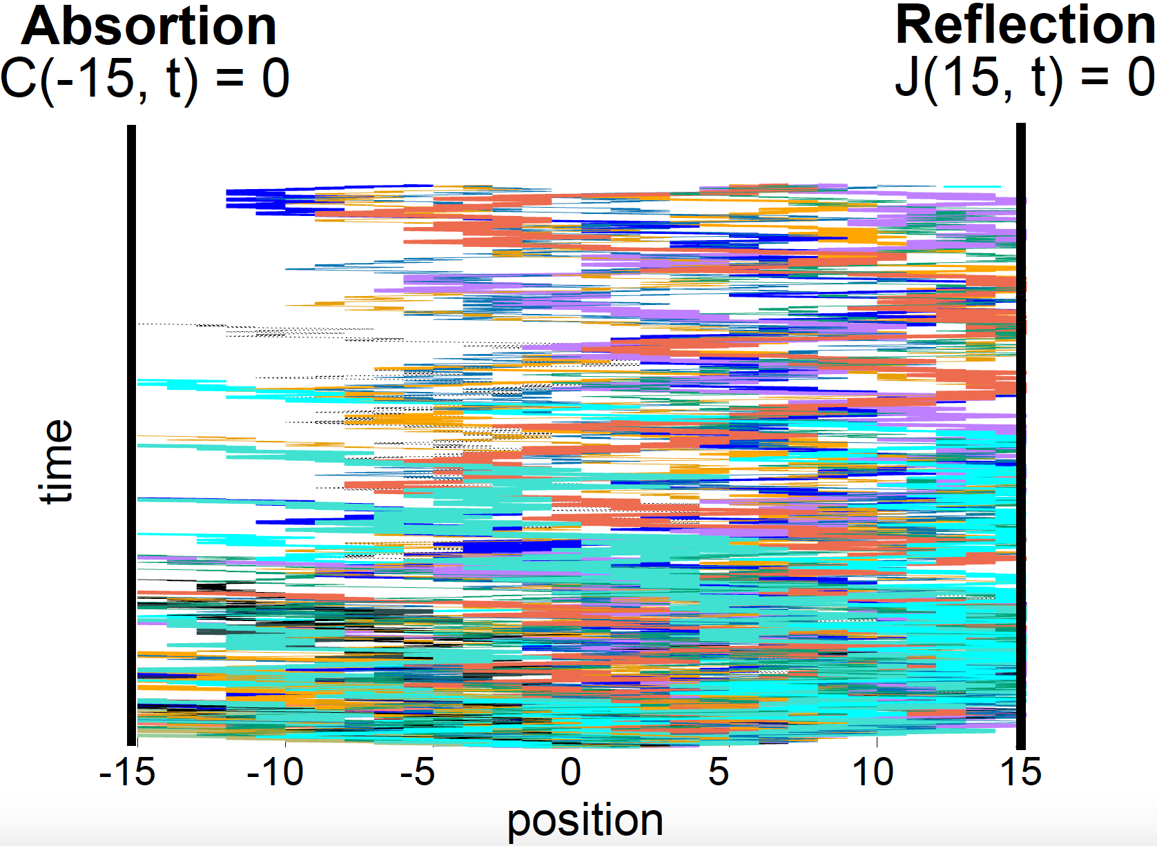
Figure 7. 1D unbiased random walks (100) with absorption at position x = -15 and reflection at position x = 15.
So far, we have assumed particles come from one source, and can move freely with no physical constraints. That is not normally the case.
- A surface at position \(x_0\) that absorbs particles is characterized by
- A surface the reflects particles is characterized by
Steady-state solutions
Steady-state solutions are those for which the concentration does not depend on time
In 1D:
\[\frac{\delta C(x,t)}{\delta t} = 0 \quad \mbox{or}\quad \frac{\delta^2 C(x,t)}{\delta x^2} = 0.\]Steady state solutions in one dimension include
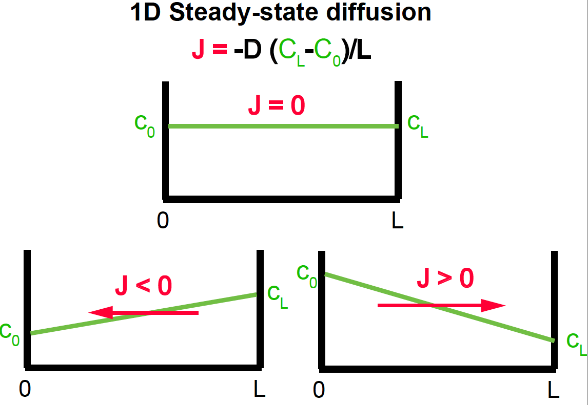
Figure 8. 1D steady-state Diffusion.
-
The concentration is constant:
\[C(x,t) = C_0,\]which results in no flux \(J(x,t) = 0.\)
-
The concentration is linear with distance
\[C(x,t) = C_0 + x \frac{C_L - C_0}{L}.\]Then the flux is constant
\[J(x,t) = -D\ \frac{C_L-C_0}{L}.\]