MCB111: Mathematics in Biology (Fall 2024)
- What is sampling?
- Why sampling?
- The cool thing we are showing here
- Some notation on PDFs and CDFs
- The CDF for the Uniform distribution
- The random variable \(F_X(X)\) is uniformly distributed
- The Inverse Transformation Method for sampling
- Indirect sampling methods
week 00:
Sampling from a probability distribution
What is sampling?
Sampling from a distribution means to take a number of data points such that their likelihood is determined by the distribution’s probability density function. As the number of samples increases, the histogram of the drawn point will increasingly resemble the original distribution.
Consider the distributions in Figure 1, you expect to see the points to start accumulating around the regions with higher probability. If the sampling continues indefinitely, you expect to eventually cover the whole sampling region. The histogram of sampled points will approximate the actual probably density function. The larger the number of points, the better the approximation.
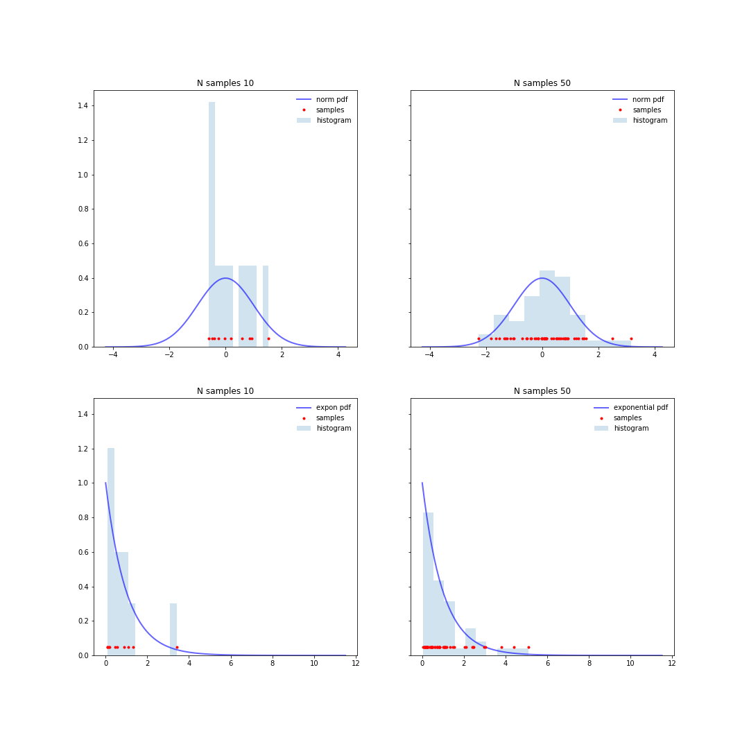
Figure 1. Top: samples for a Normal distribution. Bottom: samples for an exponential distribution. Left: 10 samples, Right: 50 samples. Sampled points are in red.
Why sampling?
Sampling from a distribution has a number of uses. One of them is to test alternative hypothesis. We do that when we want to test how data produced in an experiment fits a simpler and perhaps more boring hypothesis than the interesting hypothesis we are testing. Oftentimes the alternative hypothesis can be formulated mathematically and samples can be taken from it, and those can be compared to the actual measurements. Another use is when the probability distribution is the posterior distribution of the parameters of a model, and sampling from that distribution provides samples of models compatible with the data.
Once we have a sample \(\{x_i\}\) for a given distribution probability density \(p(x)\), then we can use those to estimate the averages of quantities derived from \(X\), \(f(x)\) as follows
\[\int f(x)\ p(x)\ dx \approx \frac{1}{N}\sum_{i=1}^N f(x_i)\]For instance, an estimation of the mean of the distribution from the sample corresponds to
\[\mu = \int x\ p(x)\ dx \approx \frac{1}{N}\sum_{i=1}^N x_i\]The cool thing we are showing here
Here we are going to show that one can produce samples from any arbitrary probability distribution just by using samples from a uniform random variable \([0,1]\).
This is an important result because even though Python has functions to generate samples from most standard probability distributions using scypy.stats, for instance, you can sample from the exponential distribution using expon.rvs, those don’t help if you have an experimentally determined probability distribution without an analytical expression.
The thing is, you only need math.random() to sample from any arbitrary distribution.
Some notation on PDFs and CDFs
For a random variable \(X\), we define the probability density function (PDF) as
\begin{equation} P(X = x) = p(x), \end{equation}
and the cumulative density function (CDF) as
\begin{equation} F_X(x) = P(X\leq x) = \int_{y\leq x} p(y)\ dy. \end{equation}
\(F_X(x)\) is the probability of getting the value \(x\) or any value smaller than it. When the PDF is high, the slope of the CDF is large, when the PDF is low, the slope of the CDF is small.
The CDF has (for a continuous variable) the following properties,
\[\lim_{x\rightarrow -\infty} F_X(x) = 0,\] \[\lim_{x\rightarrow +\infty} F_X(x) = 1.\]The CDF function \(F_X(x)\) is always increasing, that is if \(x\leq y\) then \(F_X(x)\leq F_X(y)\). Most continuous distribution are also strictly increasing, but it does not have to be that way, and it could be the case that \(F_X(x)=F_X(y)\) for \(x< y\).
Geometrically \(F_X(x)\) is the area under the curve of \(P(X)\) up to \(x\). See Figure 2. And we can see that
\[P(a\leq x \leq b) = F_X(b) - F_X(a).\]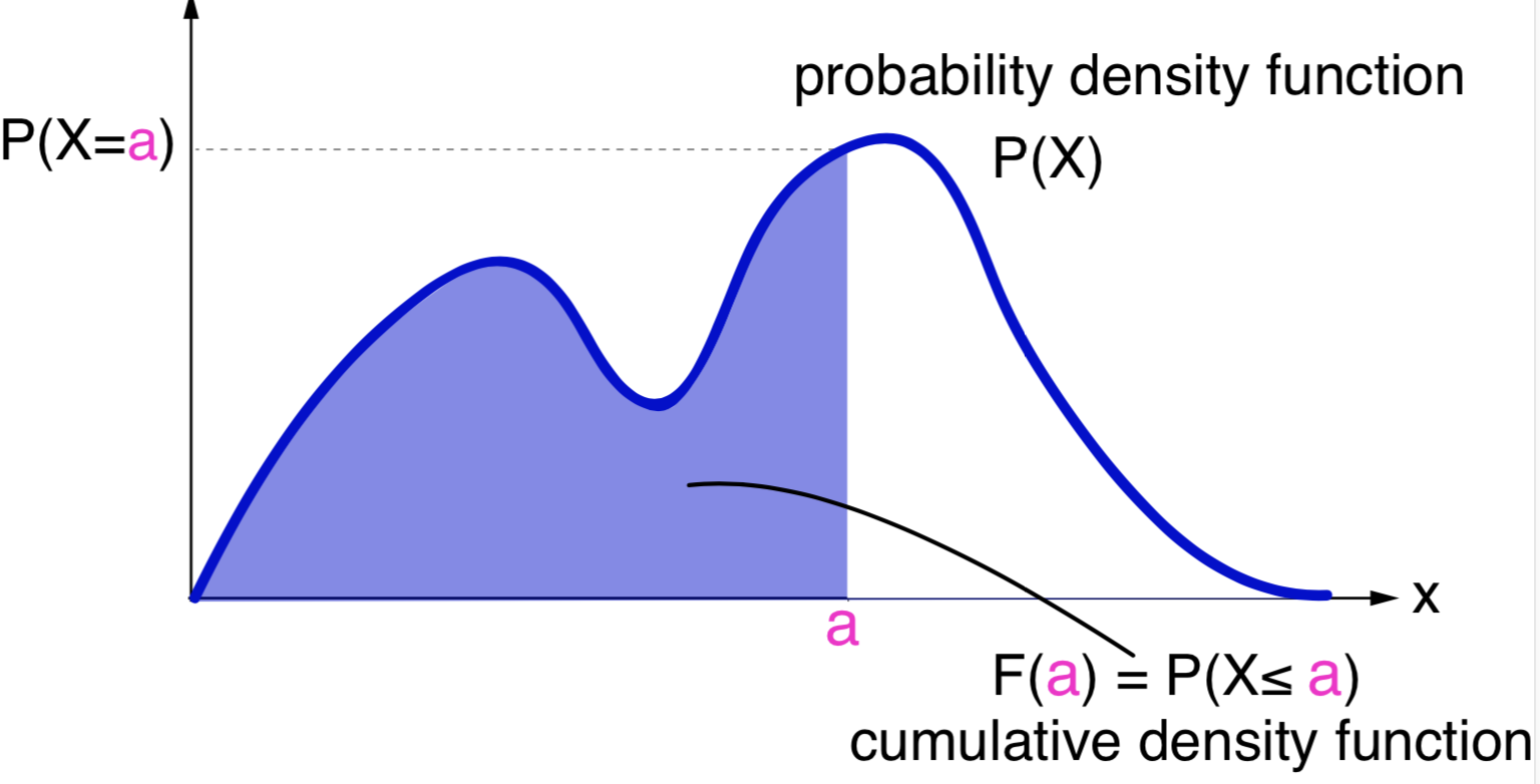
Figure 2. Relationship between the probability density function (PDF) and the cumulative density function (CDF).
The CDF for the Uniform distribution
Let’s take a moment to remind ourselves of an important property of the Uniform distribution.
A uniform random variable \(U(a,b)\) on \([a,b]\) is such that the PDF is given by
\[\begin{equation} P(U=x) = \begin{cases} 0 & \mbox{if}\quad x < a\\ \frac{1}{b-a} & \mbox{if}\quad a\leq x \leq b\\ 0 & \mbox{if}\quad x > b \end{cases} \end{equation}\]And the CDF is given by
\[\begin{equation} F_U(x) = P(U\leq x) = \int_{-\infty}^{x} P(U=y)\ dy = \begin{cases} 0&\mbox{if}\quad x < a\\ \frac{x-a}{b-a}&\mbox{if}\quad a\leq x \leq b\\ 1&\mbox{if}\quad x > b \end{cases} \end{equation}\]And in the particular case of a uniform random variable \(U\) on \([0,1]\), we have the results
\[\begin{equation} F_U(x) = \begin{cases} 0&\mbox{if}\quad x < 0\\ x&\mbox{if}\quad 0\leq x \leq 1\\ 1&\mbox{if}\quad x > 1 \end{cases} \end{equation}\]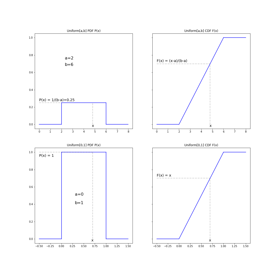
Figure 3. The Uniform distribution. (left) the probability density function (PDF), (right) the cumulative density function (CDF)
That is, if we sample a number \(r\in[0,1]\) using a random number generator, such as random.random(), we have that
\[F_U(r) = P(U\leq r) = r.\]In particular, because for any CDF, \(F_X(X)\) takes values in \([0,1]\) then we have,
\[P(U \leq F_X(x)) = F_X(x).\]This apparently trivial result is at the core of the Inverse Transformation method for sampling that we discuss next.
The random variable \(F_X(X)\) is uniformly distributed
For any random variable \(X\) that follows the probability distribution \(P(X)\), such that \(F_X(x) = P(X\leq x)\), we can show that \(F_X(X)\) is the uniform distribution U in \([0,1]\).
What does this mean?
It means that if \(x_1,\ldots, x_N\) is a sample from a probability distribution with CDF \(F_X\), then the sample given by
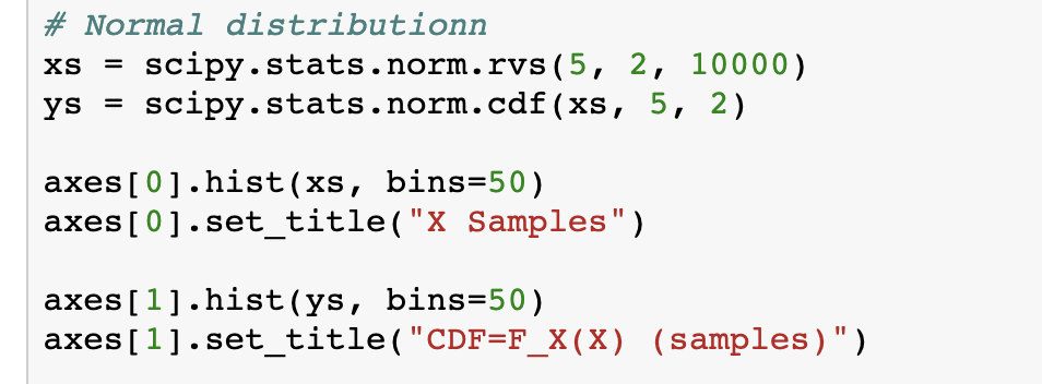
follows a uniform distristribution in \([0,1]\).
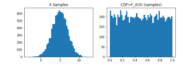
Figure 4.
In python pseudo code
Produces the result in Figure 4.
Proof
Introduce \(Z=F_X(X)\). Then for the CDF of Z we have,
\[F_Z(x) = P(F_X(X) \leq x) = P(X\leq F_X^{-1}(x)) = F_X(F_X^{-1}(x)) = x.\]Thus, \(Z=F_X(X)\) is the uniform distribution in \([0,1]\).`
We will also use this result later in the course when we discuss p-values. After all, a p-value is a CDF (or \(1-CDF\) more precisely), which means that p-values are uniformly distributed. We will discuss the implications of that fact.
The Inverse Transformation Method for sampling
This method allows us to sample from an arbitrary probability distribution using only a random number generator that samples uniformly on \([0,1]\).
How it works
The Inverse Transformation method just requires to sample a value \(r\) from the Uniform distribution on \([0,1]\), and to take \(x=F_X^{-1}(r)\) as the sampled value.
In practice, it requires to have the cumulative distribution function and
- Generate a uniformly distributed sample \(r\) in \([0,1]\).
- Visualize a horizontal line to the CDF.
- Output index of the intersection as a sample.
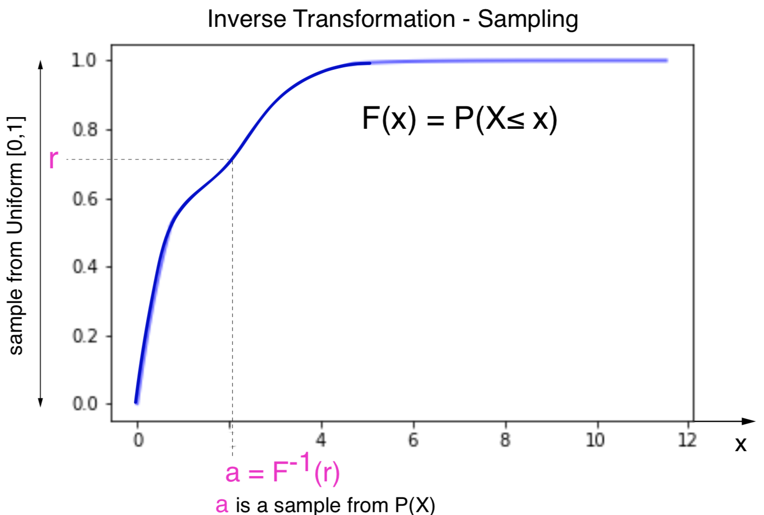
Figure 5. Graphical representation of the Inverse transformation sampling methods
Notice that for this Inverse Transformation to work, the CDF \(F_X\) has to be invertible, which requires that if \(x< y\) then \(F_X(x) < F_X(y)\), but not \(F_X(x) = F_X(y)\), in which case the inverse would not be possible to calculate.
Why it works
We want to show that \(P(X\leq x)\) when \(x = F_X^{-1}(r)\) and \(r\) has been sampled uniformly in \([0,1]\) is indeed \(F_X(x)\).
Introduce the random variable \(A = F_X^{-1}(U)\) , we want to show that \(A=X\).
\[F_A(x) = P(A \leq x) = P (F_X^{-1}(U) \leq x)\]Because \(F_X^{-1}(U) = X\) means that \(U = F_X(X)\), then
\[P(A \leq x) = P (F_X^{-1}(U) \leq x) = P(U\leq F_X(x)) = F_X(x),\]where the last equalty is the result of the property we show before for the Uniform distribution, so that \(A = X\).
where for the last step, I have used the property that we found for the uniform distribution in the previous section, and described in the bottom right plot in Figure 2.
Example: sampling from an Exponential Distribution
The exponential distribution is one of the few cases of a distribution for which the CDF \(F_E\) has an inverse \(F^{-1}_E\) with an analytic expression.
The exponential distribution describes processes that occur randomly over time with a fixed rate \(\lambda\). The exponential distribution is widely used in biology to describe decay processes such as RNA or protein degradation for instance.
The PDF of the exponential distribution is given by
\[P(E=x) = \lambda\ e^{-\lambda x},\]where \(\lambda > 0\) is an arbitrary parameter, and the range of \(x\) is \([0,\infty)\).
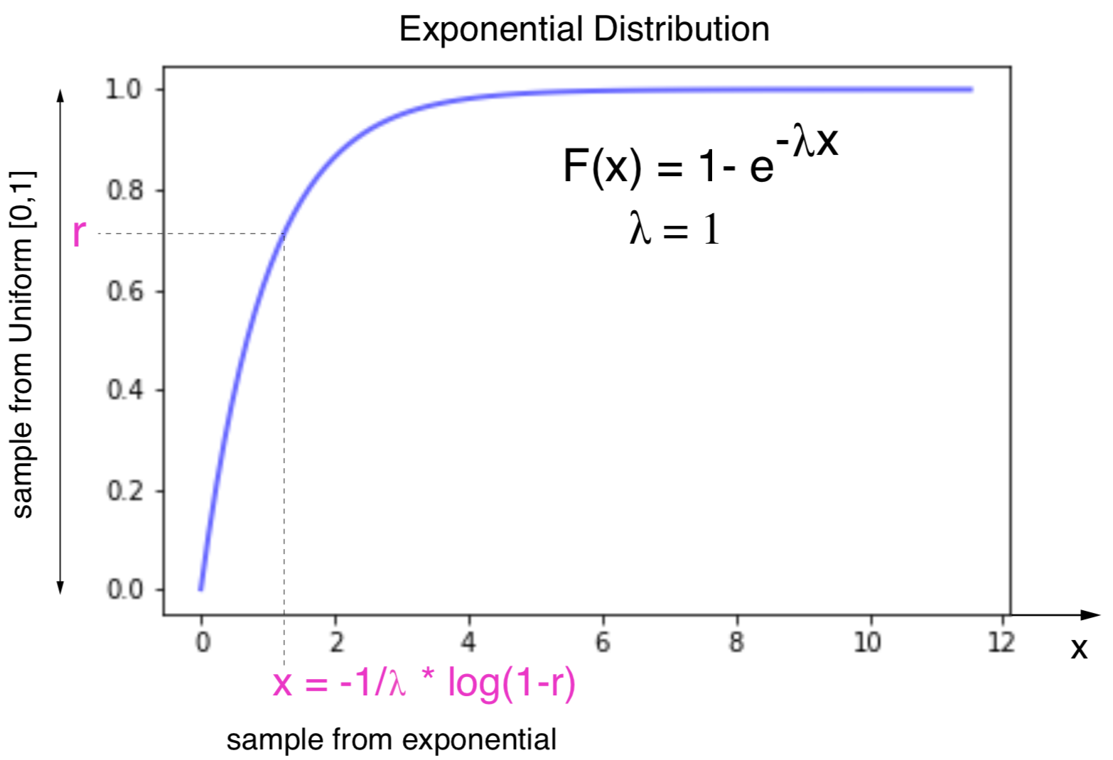
Figure 6. Inverse sampling for the exponential distribution.
The CDF can be calculated analytically as
\[F_E(x) = \int_{-\infty}^x \lambda e^{-\lambda y}\ dy = -e^{-\lambda y}\mid_{\infty}^x = -e^{-\lambda x} + 1 = 1 - e^{-\lambda x}.\]For a value \(r_i\) sampled uniformly in \([0,1]\), a \(x_i\) sampled according to the exponential distribution can be obtained using the expression,
\[r_i =1 - e^{-\lambda x_i}\]that is
\[1 - r_i = e^{-\lambda x_i}\]or
\[log(1-r_i) = -\lambda x_i\]finally
\[x_i = -\frac{1}{\lambda}\log(1-r_i) = F_E^{-1}(r_i).\]In summary, to sample from an exponential distribution can be obtained from uniformly sampled values \(r_i\) on \([0,1]\) as
\[-\frac{1}{\lambda}\log(1-r_i)\]Notice that the sampled values are positive as \(log(1-r) < 0\) if \(0<r<1\),
Indirect sampling methods
The Inverse Transformation Method directly samples from the distribution \(p(x)\). In some cases, \(p(x)\) is not available, and several algorithms have been designed to sample when directly sampling from \(p(x)\) is not possible.
Rejection sampling
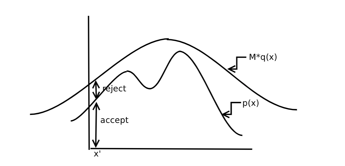
Figure 7. Rejection sampling
To sample from a probability density \(p(x)\) is to sample uniformly the area under the curve. In rejection sampling, you sample the area under a different density \(q(x)\), with the restriction that \(p(x) \leq M*q(x)\), see Figure 7 from “MonteCarlo Sampling” by M I Jordan.
To generate a sample from \(p(x)\),
-
sample \(x_i\) in \(q(x)\)
-
sample \(r\) uniformly in \([0,1]]\)
-
then, \(\begin{equation} \begin{cases} \mbox{if}\, r < \frac{p(x_i)}{M*q(x_i)} &\mbox{accept}\quad x_i\\ \mbox{else} &\mbox{reject}\quad x_i\\ \end{cases} \end{equation}\)
In regions where \(p(x)\) is high, we are less likely to reject a sample \(x\), and we will get more values in that region.
This method we may waste a lot of time rejecting samples if the distribution has many peaks and valleys.
Importance sampling
Importance sampling is used when sampling from a given distribution with density \(p(x)\) is very difficult, but there is a related distribution \(g(x)\) from which it is easier to sample.
Importance sampling does not allow to calculate directly samples of \(p(x)\), but it can be used to calculate averages of an arbitrary function \(f(x)\) respect to the density \(p(x)\).
\[\langle f\rangle = \int f(x)\ p(x)\ dx,\]which can be expressed using the auxiliary distribution \(g(x)\) as
\[\langle f\rangle_p = \int f(x)\ p(x)\ dx = \int f(x)\ \frac{p(x)}{g(x)}\ g(x)\ dx= \int f(x)\ w(x)\ g(x)\ dx = \langle f*w\rangle_g\,\]where the weights are defined as \(w(x) = \frac{p(x)}{g(x)}.\)
The importance sampling method goes as follows
-
Take N samples \(\{x_i\}_{i=1}^N\) from \(g(x)\)
-
calculate the weights \(w(x_i) = \frac{p(x_i)}{g(x_i)}\)
-
estimate \(\langle f\rangle \approx \frac{1}{N} \sum_if(x_i)\ w(x_i).\)
Monte Carlo sampling
Monte Carlo sampling is a very generic term to describe any method that allows you to approximate a probability distribution \(p(x)\) by taking a number of samples \(\{x_i\}\), such that for any function \(f(x)\) of the random variable you can use,
\[\int f(x)\ p(x)\ dx \approx \frac{1}{N}\sum_{i=1}^N f(x_i).\]Many difference techniques or “sampling rules” can be used to produce those samples \(\{x_i\}\) representatives of \(p(x)\).
Rejection sampling and Importance sampling are examples of Monte Carlo sampling. Another well known method is Markov Chain Monte Carlo (MCMC), in which the sampling rule is a Markov process (that is, a process that depends only on the previously sampled value).