MCB111: Mathematics in Biology (Fall 2024)
- What is information content, and how to measure it
- Information, Redundancy and Compression
- Entropy: the average information content of an ensemble
- Relative entropy: the Kullback-Leibler divergence
- Mutual Information
- The principle of maximizing entropy. Or trusting Shannon to be fair
week 01:
Introduction to Information Theory
For this topic, you will probably find relevant MacKay’s book (Sections 2.4, 2.5, 2.6), and also MacKay’s lecture 1 and lecture 2 from his online ``Course on Information Theory, Pattern Recognition, and Neural Networks’’, from which I have borrowed a lot of the language.
Here is another set of related materials “Visual Information Theory”. I don’t follow it directly, but it covers many of the same basic topic, with very explicit visualizations. If you find my notes or MacKay’s book difficult to follow, you should definitely check this reference out. We don’t all learn the same way.
What is information content, and how to measure it
The term information content was introduced by Claude Shannon (1916-2001) in his 1948 landmark paper “A Mathematical Theory of Communication” to solve communication problems. With this paper, Shannon founded the field of Information Theory. I strongly recommend that you look at the actual paper. It’s a long paper, pages 1 and 2, and Section 6 (“Choice, uncertainty and entropy”, page 14) are a good start for what we will discuss in this lecture.
As a side, I also recommend that you learn about Shannon’s closest collaborator Betty Moore Shannon.
The problem was how to obtain “reliable communication over an unreliable channel”.
Examples relevant to you can be:
- voice \(\rightarrow\) ear (channel = air)
- DNA \(\rightarrow\) DNA replication (channel = DNA polymerase)
- biological system perturbation \(\rightarrow\) measurement (channel = your experimental design)
The received signal is never identical to the sent signal. How can we make it so the received message is as similar as possible to the sent message?
For the case of your biological experiment, you could either
- Improve the experiment
- Add redundancy (Hamming codes).
Properties of information content
Information content is inversely related to how frequent an event is
Consider these examples. We barely know each other, I run into you and I say:
- I had breakfast this morning,
- Today is not my birthday,
- Today is my birthday,
- I ran the first (2016) Cambridge half-marathon,
- I ran the first and second Cambridge half-marathons,
- I ran the first, second and third Cambridge half-marathons,
- I have been to Antarctica,
Which of these events you think carries the most information? (Disclaimer: not all events directly apply to me.)
The information conveyed by one event is ‘somehow’ inversely related to how frequent that event is (we will specify the ‘how’ later). And often times, how frequent an event is depends on the number of possible outcomes. Such that,
-
The rarer an event is, the lower its probability, and the more information you could transmit by running the experiment (listening at the end of the channel).
-
Equivalently, the more ignorant you are about the outcome (because the number of possibilities is very large), the smaller the probability of each individual outcome, and the more information you could get from listening at the end of the channel.
Thus, for an event \(e\) that has probability \(p\), we expect that
\begin{equation} \mbox{the Information_Content} (e)\quad \mbox{grows monotonically as 1/p.} \end{equation}
Information content is additive
A second desired property of information is that, for two independent events \(e_1\) and \(e_2\), we expect the total information to be
\begin{equation} \mbox{Information_Content} (e_1 \& e_2) = \mbox{Information_Content} (e_1) + \mbox{Information_Content} (e_2). \end{equation}
Ta-da!
Using these two desirable properties for information content, we can derive its mathematical form.
The logarithm function has the convenient property:
\begin{equation} \log(ab) = \log(a) + \log(b). \end{equation}
Shannon postulated that, for an event \(e\) that has probability \(p\), the right way of measuring its information is,
\begin{equation} \mbox{Information Content}(e) = h(e) = \log_2 \frac{1}{p} \quad \mbox{in bits.} \end{equation}
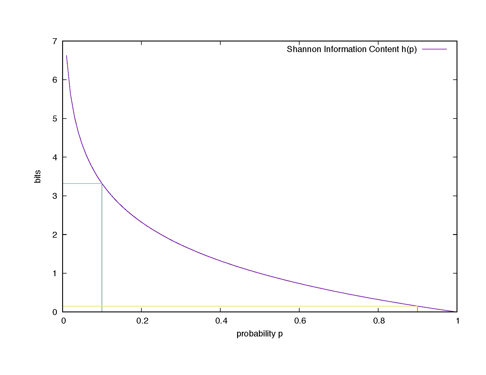
Figue 1. Shannon information content as a function of the probability value. Examples: h(p=0.1) = 3.32 bits, h(0.9)= 0.15 bits.
In Figure 1, we see how information content varies as a function of the probability. Going back to my examples,
| Event | Probability | Entropy (bits) |
|---|---|---|
| I had breakfast today | 1.0 | 0.0 |
| Today is not my birthday | 364/365 | 0.004 |
| Today IS my birthday | 1/365 | 8.5 |
| Ran first Cambridge half-marathon | 4,500/4,700,000\(^\ast\) | 10.0 |
| Ran first & second Cambridge half-marathon | (4,500/4,700,000)x(6,500/4,700,000)\(^{\ast\ast}\) | 13.5 |
| I’ve been to Antarctica | 925,000/7,400,000,000\(^{+}\) | 13.0 |
| I’ve lived in Antarctica in winter (June) | 25,000/7,400,000,000\(^{++}\) | 18.2 |
\(^{\ast}\)I have considered the greater Boston population (4.7 millions).
\(^{\ast\ast}\)I have assumed that the two events (running the first and second half-marathon) are independent, but in fact they aren’t.
\(^{+}\)Tourists to Antarctica in 2009-2010 season amounted to 37,000. I have considered 25 years of visits (since the 1990s).
\(^{++}\) About 1,000 people live in Antarctica in winter. I have considered 25 years of Antarctica colonization.
Do these results agree with your intuition about how much you learned about me by knowing those facts?
Let’s see how additivity for the information of two independent events works
For two independent events \(e_1\) and \(e_2\),
\begin{equation} P(e_1,e_2) = P(e_1)P(e_2), \end{equation}
then
\begin{eqnarray}
h(e_1 \& e_2)
&=& \log_2 \frac{1}{P(e_1,e_2)}
&=& \log_2 \frac{1}{P(e_1)P(e_2)}
&=& \log_2 \frac{1}{P(e_1)} + \log_2 \frac{1}{P(e_2)}
&=& h(e_1) + h(e_2).
\end{eqnarray}
Note about the log scale
You can define entropy using any logarithm base you want.
- If I say \(I = \ln(\frac{1}{p})\quad\quad\) I am measuring entropy in nats
- If I say \(I = \log_{2}(\frac{1}{p})\quad\) I am measuring entropy in bits
- If I say \(I = \log_{10}(\frac{1}{p})\quad\) I am measuring entropy in base 10
The relationship is
\[\begin{aligned} \ln(a) &= b\quad\,\,\,\ \mbox{means}\quad a = e^{b}\\ \log_2(a) &= b_2\quad\,\, \mbox{means}\quad a = 2^{b_{2}}\\ \log_{10}(a) &= b_{10}\quad \mbox{means}\quad a = 10^{b_{10}}\\ \log_{n}(a) &= b_{n}\quad\,\ \mbox{means}\quad a = n^{b_{n}} \quad\mbox{for an arbitrary base}\, n\\ \end{aligned}\]Then
\[e^{b} = 2^{b_{2}} = 10^{b_{10}} = n^{b_n},\]Thus, the relationship between natural logs and logs in any other base \(n\) is
\[b = \ln(n^{b_n}) = b_n\ln(n).\]In particular, the relationship between nats and bits is
\[b_{\mbox{nats}} = b_2\ \ln(2).\]In general, I will use \(\log(x)\) interchangeably with \(\ln(x)\) to refer to natural logs. If I don’t specify a base, I am using natural logs.
Information, Redundancy and Compression
The information content is inversely related to redundancy. The less information an event carries, the more it can be compressed.
Shannon postulated that, for an event \(e\) of probability \(p\), its information content is the compression to which we should aspire.
Entropy: the average information content of an ensemble
The entropy of a random variable X is the average information content of an ensemble of all the possible outcomes (variables) for X,
\begin{equation} \mbox{Entropy}(X) = H(X) = \sum_x p(x) \log \frac{1}{p(x)}, \end{equation}
with the convention that if \(p(x) = 0\), then \(0\times \log\frac{1}{0} = 0\).
Notice that the entropy is never negative, \begin{equation} H(X) \geq 0, \end{equation}
with
\begin{equation} H(X) = 0\quad\mbox{ if and only if}\quad p(x)=1 \quad\mbox{for one}\quad x. \end{equation}
A desirable property of H that Shannon describes in his classical paper is that if a choice is broken down in two different choices the original H should be the weighted sum of the individual entropies. Graphically, using Shannon’s own figure
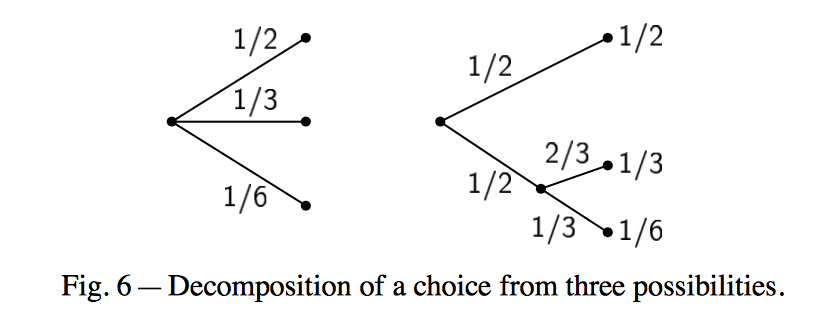
We have the equality,
\[H\left(\frac{1}{2},\frac{1}{3},\frac{1}{6}\right) = H\left(\frac{1}{2},\frac{1}{2}\right) + \frac{1}{2} H\left(\frac{2}{3},\frac{1}{3}\right).\]The coefficient \(\frac{1}{2}\) weights the fact that the second choice only happens half of the time.
Relative entropy: the Kullback-Leibler divergence
For two probability distributions \(P(x)\) and \(Q(x)\) defined over the same space, their relative entropy or Kullback-Leibler (KL) divergence is defined by
\[D_{KL}(P||Q) = \sum_x P(x)\, \log{\frac{P(x)}{Q(x)}}.\]The relative entropy has the following properties
-
It satisfies Gibbs’s inequality
\[D_{KL}(P||Q) \geq 0.\]It is zero only if \(P=Q\).
-
It is not symmetric. In general,
\[D_{KL}(P||Q) \neq D_{KL}(Q||P).\]Thus, it is not a distance although oftentimes it is called the KL distance.
-
For continuous distributions it takes the form
\[D_{KL}(P||Q) = \int_x p(x)\, \log{\frac{p(x)}{q(x)}}\, dx,\]where \(p(x)\) and \(q(x)\) are the densities of \(P\) and \(Q\).
Mutual Information
Mutual Information is a particular case of relative entropy.
For two random variables \(X\) and \(Y\), with join probability distribution \(P_{XY}\), and marginal probability distributions \(P_X\) and \(P_Y\), we define the mutual information as
\[MI(X,Y) = D_{KL}(P_{XY}||P_X P_Y) = \int_x\int_y p(x,y)\, \log{\frac{p(x,y)}{p(x)p(y)}}\, dx\, dy,\]Mutual information measures how different the random variables \(X, Y\) are from being independent of each other.
The principle of maximizing entropy. Or trusting Shannon to be fair
Imagine you have 8 pieces of cake that you want to distribute amongst 3 kids, without cutting the pieces further. How would you do that? Unless you are Gru (despicable me), you would like to be as fair as possible to all three kids.
Here are some options. Would you give?
- 4 4 0
- 4 2 2
- 3 3 2
Then entropy of these three different scenarios are
- \(H(4,4,0) = 1.00\) bits
- \(H(4,2,2) = 1.50\) bits
- \(H(3,3,2) = 1.56\) bits
Do these entropy values correlate with your gut feel about fairness?
In the same way, when you are working in an experiment for which you expect different possible outcomes, but you have no idea of which are more favorable, being fair to all of them (that is, not giving preference to each) you should also use the maximum entropy principle.
The maximum entropy distribution is the one that favors any of the possible outcomes the least. Thus, the maximum entropy distribution is the one that should be used in the absence of any other information.
The principle of maximal entropy was introduced by E.T. Jaynes in his 1957 paper “Information theory and statistical mechanics.
Still in the issue of being fair to the 3 kids and the 8 pieces of cake, now consider this option in which you give 2 pieces to each kids and leave 2 pieces out:
\begin{equation} H(2,2,2) = \frac{2}{6}\log_2\frac{1}{2/6} + \frac{2}{6}\log_2\frac{1}{2/6} + \frac{2}{6}\log_2\frac{1}{2/6} = \log_2(3) = 1.59 \, \mbox{bits}. \end{equation}
What do you think about this result? This entropy is even higher than the (3,3,2) case that seemed pretty fair. How come?
You can formally ask, what is the probability distribution that maximizes the entropy of the system? This is an optimization problem.
Maximum-entropy estimates
In Section 2, Jaynes establishes the properties of maximum-entropy inference. Following Jaynes, I will assume a discrete distribution, but it works as well for any continuous distribution.
The random variable \(X\) takes discrete values \(\{x_1,\ldots , x_n\}\), but we don’t know the probability distribution
\begin{equation} p_i = P(x_i)\quad\quad \sum_{i=1}^n p_i = 1. \end{equation}
The only thing we know is the expected value of a particular function \(f(x)\), given by
\begin{equation} \sum_{i=1}^n f(x_i)\ p_i = {\hat f}. \end{equation}
Using only this information, what can we say about \(p_i\)?
The maximum-entropy principle says that we need to maximize the entropy of the probability distribution
\begin{equation} H(p_1\ldots p_n) = -\sum_i p_i\ \log p_i, \end{equation}
subject to the two constraints,
\[\begin{aligned} \sum_i p_i &= 1,\\ \sum_i f(x_i)\ p_i &= {\hat f}. \end{aligned}\]We solve such constrained optimization problem by introducing one Lagrange multiplier for each constraint (\(\lambda\) and \(\lambda_f\)), such that the function to optimize is give by
\begin{equation} L = -\sum_j p_j \log{p_j} -\lambda \left(\sum_j p_j - 1\right) - \lambda_f \left(\sum_j p_j\ f(x_j) - {\hat f}\right). \end{equation}
The derivative respect to one such probability \(p_i\) is
\begin{equation} \frac{d}{d p_i} L = -\log{p_i} - p_i \frac{1}{p_i} - \lambda -\lambda_f f(x_i), \end{equation}
which becomes optimal when \(\frac{d}{d p_i} L = 0\), then
\begin{equation} \log{p^{\ast}_i} = -\left[1 + \lambda + \lambda_f\ f(x_i)\right], \end{equation}
or
\begin{equation} p^{\ast}_i = e^{-\left[1+\lambda + \lambda_f\ f(x_i)\right]}. \end{equation}
Because \(\sum_i p_i = 1\), that implies that
\[1 = e^{-(1+\lambda)} \sum_i e^{-\lambda_f\ f(x_i)}\]And the maximum-entropy probability distribution is given by
\begin{equation} p^{\ast}_i = \frac{e^{-\lambda_f\ f(x_i)} }{\sum_j e^{-\lambda_f\ f(x_j)} }. \end{equation}
This result generalizes for any number of functions \(f_r\) for which we know their averages
\[\sum_i f_r(x_i)\ p_i = {\hat f_r}\]the maximum-entropy probability distribution is given by
\begin{equation} p^{\ast}_i = \frac { e^{-\left[\lambda_1\ f_1(x_i) +\ldots + \lambda_m\ f_m(x_i)\right]} } { \sum_j e^{-\left[\lambda_1\ f_1(x_j)+\ldots + \lambda_m\ f_m(x_j)\right]} }. \end{equation}
Paraphrasing Jaynes, the maximum-entropy distribution has the important property that no possible outcome is ignored. Every situation that is not explicitly forbidden by the given information gets a positive weight.
Particular maximum-entropy distributions are:
When you do not know anything about the distribution
In the particular case in which we don’t even know the average of any value,
\[f=0\]then, the equation above becomes
\begin{equation} p^{\ast}_i = \frac{1}{N}, \quad \mbox{for}\quad 1\leq i\leq N. \end{equation}
That is, the maximum-entropy distribution in the absence of any information is the uniform distribution
Notice that in the case of the three kids each with 2 pieces of cake, we used a uniform distribution.
We could have done the same for a continuous distribution in a range \([a,b]\), then the maximum entropy uniform distribution looks like \begin{equation} p(x) = \frac{1}{b-a}, \quad \mbox{for}\quad x\in [a,b], \end{equation} such that, \(\int_{x=a}^{x=b} p(x) dx = 1\).
When you know the mean
When you know the mean (\(\mu\)) of the distribution, that is, the function is
\[f(x) = x,\]and you know that
\[\int f(x)\ p(x) = \int x\ p(x) = \mu\]The maximum-entropy solution when you know the mean of the distribution is given by an exponential distribution
\begin{equation} p^\star(x) = \frac{e^{-\lambda_{\mu}\ x}}{\int_y e^{-\lambda_{\mu}\ y}} \end{equation}
The value of \(\lambda_{\mu}\) can be determined using the condition
\[\mu = \int_x x\ p^\ast(x) dx = \frac{\int_x x e^{-\lambda_{\mu}\ x}}{\int_y e^{-\lambda_{\mu}\ y}}\]So far, we have said nothing about the range of x. This equation has a solution only if all x are positive.
Now, we remember that \begin{equation} \int_0^{\infty} e^{-\lambda_{\mu} x} dx = \frac{1}{\lambda_{\mu}} \end{equation}
and
\begin{equation} \int_0^{\infty} x\, e^{-\lambda_{\mu} x} dx = \frac{1}{\lambda_{\mu}^2}. \end{equation}
(You can find these results in the Spiegel manual, (equation 18.76)).
The solution is \begin{equation} \mu = \frac{1/\lambda_{\mu}^2}{1/\lambda_{\mu}} = \frac{1}{\lambda_{\mu}}. \end{equation}
Thus, the exponential distribution \begin{equation} p(x) = \frac{1}{\mu} e^{-x/\mu} \quad x\geq 0, \end{equation} is the maximum entropy distribution amongst all distributions in the \([0,\infty)\) range that have mean \(\mu\).
When you know the standard deviation
If what we know is the variance of the distribution (\(\sigma^2\)), that is, the function is
\[f(x) = (x-\mu)^2,\]and you know that
\[\int f(x)\ p(x) = \int (x-\mu)^2\ p(x) = \sigma^2\]then
\begin{equation} p^{\ast}(x) = \frac{e^{-(x-\mu)^2\lambda_{\sigma}}}{\int_y e^{-(y-\mu)^2\lambda_{\sigma}} dy}, \end{equation}
that is the maximum-entropy distribution when you know the variance is the Gaussian distribution.
The value of \(\lambda_{\sigma}\) can be determined using the condition \begin{equation} \sigma^2 \equiv \int_x (x-\mu)^2 p(x) dx = \frac{\int_x (x-\mu)^2 e^{-(x-\mu)^2\lambda_{\sigma}} dx}{\int_y e^{-(y-\mu)^2\lambda_{\sigma}} dy}. \end{equation}
Now, we remember that
\begin{equation} \int_{-\infty}^{\infty} e^{-(x-\mu)^2\lambda_{\sigma}} dx = \sqrt{\frac{\pi}{\lambda_{\sigma}}} \end{equation} and \begin{equation} \int_{-\infty}^{\infty} (x-\mu)^2 e^{-(x-\mu)^2\lambda_{\sigma}} dx = \sqrt{\frac{\pi}{\lambda_{\sigma}}} \frac{1}{2\lambda_{\sigma}}. \end{equation}
(You can find these results in the Spiegel manual, (equation 18.77)).
The solution is \begin{equation} \sigma^2 = \frac{1}{2\lambda_{\sigma}}. \end{equation}
Thus, the Gaussian distribution
\begin{equation} p(x) = \frac{1}{\sqrt{\pi/\lambda_{\sigma}}}\ e^{-(x-\mu)^2\lambda_{\sigma}} = \frac{1}{\sqrt{2\pi\sigma^2}}\ e^{-\frac{(x-\mu)^2}{2\sigma^2}}, \end{equation}
is the maximum entropy distribution amongst all distributions in the \((-\infty,\infty)\) range that have variance \(\sigma^2\).
In summary, when you want to model a set of observations with a probability distribution, them maximum entropy principle tells you that if you don’t know anything about the probability of the different outcomes, you should use a uniform distribution, if you know the mean, the maximum entropy distribution is an exponential distribution, and if you know the standard deviation the maximum entropy distribution is the Gaussian distribution.