week 13:

Diffusion-Reaction patterns

Preliminars

Present all your reasoning, derivations, plots and code as part of the homework. Imagine that you are writing a short paper that anyone in class should to be able to understand. If you are stuck in some point, please describe the issue and how far you got. A jupyter notebook if you are working in Python is not required, but recommended.

The Brusselator on steroids

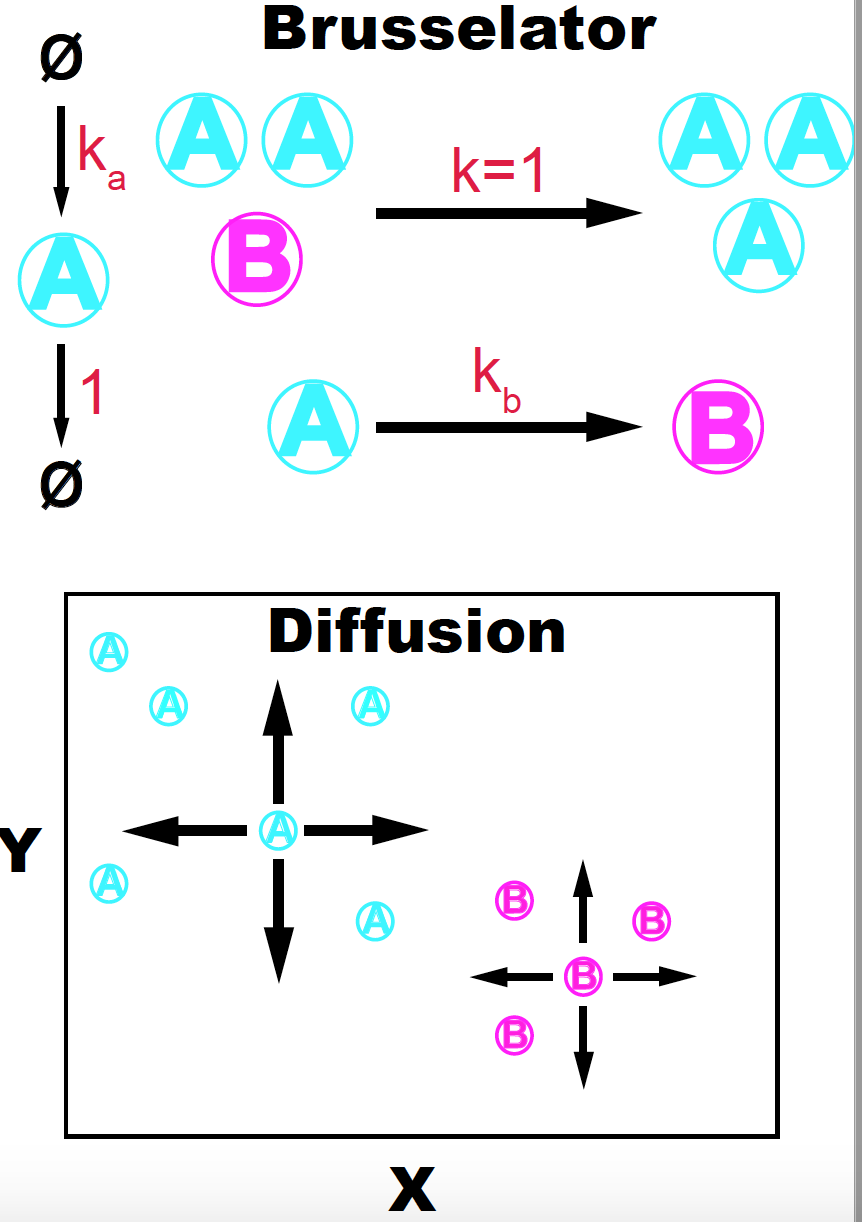
Figure 1. The Brusselator + diffusion model. Adapted from K. Sims (http://www.karlsims.com/rd.html).

In class, we showed how the Gray-Scott model is a two-species system that in two dimensions can produce striking spatial patterns. Here, we are going to look at another two-species model that also produces interesting patters.

The Brusselator is just a theoretical model, and it got its name because it was proposed by investigators at the Universite libre de Bruxelles. The Brusselator is a purely reaction process, and it is interesting on its own because it can produce oscillations, thus the name Brusselator.

These are the reactions that define the Brusselator. There are two species \(A\) and \(B\) such that,

\[\begin{aligned} A\overset{k_b}{\longrightarrow} B\\ 2A+ B\overset{k=1}{\longrightarrow} 3 A\\ \emptyset \overset{k_a}{\longrightarrow} A\\ A \overset{1}{\longrightarrow} \emptyset, \end{aligned}\]

that is, \(A\) transforms to \(B\), and \(B\) transforms to \(A\) but this last reaction can only occur in the presence of two additional \(A\) molecules

But here, we are not going to study the Brusselator reactions alone, but the result of combining the Brusselator with a diffusion process. The \(A\) and \(B\) in addition to being subject to the Brusselator’s reactions, they can diffuse in both the \(x\) and \(y\) directions with diffusion coefficients \(D_A\) and \(D_B\) respectively.

We will workout this exercise in class, but that we need to do is

Write the continuous differential equations associated to the Brusselator + diffusion model in two spatial directions \(x\) and \(y\).
Find the steady state(s) of the Brusselator (sans diffusions).
Implement the code to solve the equations numerically.
Make patterns!

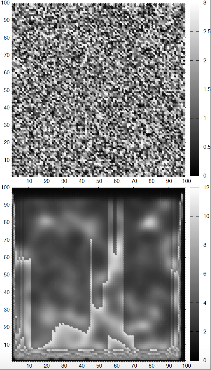
Figure 2. Brusselator-diffusion patterns. The top figure depicts the initial conditions for species A. The bottom figure depicts the concentration of A after some time. Parameters values are described in the text. The concentration of species B is a mirror image of that of A.

Do not forget the four conditions necessary to convert the system from a steady state of the Brusselator alone, into pattern-forming when including the diffusion terms,

\[F^\ast_{AA} + F^\ast_{BB} < 0\\ F^\ast_{AA} F^\ast_{BB} - F^\ast_{AB} F^\ast_{BA} > 0\\ D_B F^\ast_{AA} + D_A F^\ast_{BB} > 0\\ D_B F^\ast_{AA} + D_A F^\ast_{BB} > 2 \sqrt{D_A D_B (F^\ast_{AA} F^\ast_{BB} - F^\ast_{AB} F^\ast_{BA})}\]

where \(A^\ast, B^\ast\) is a steady state of the Brusselator alone.

Here are some possible sets of parameters and initial conditions that in my hands produced cool patterns. I used a square of length \(L = 100\), and \(\Delta x = 0.5\). I run it until \(T=1,500\), with \(\Delta t = 0.05\).

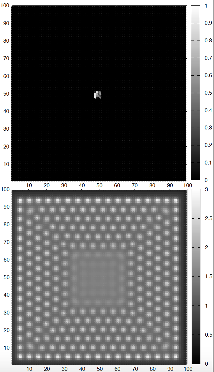
Figure 3. Brusselator-diffusion patterns. The top figure depicts the initial conditions for species A. The bottom figure depicts the concentration of A after some time. Parameters values are described in the text. The concentration of species B is a mirror image of that of A.

Figure 2
\[\begin{aligned} k_a &= 3\\ k_b &= 9\\ D_A &= 5\\ D_B &= 12 \end{aligned}\]
The initial conditions are very important. Different initial conditions can change the resulting patterns significantly for the same underlying reactions. In Figure 2, The square was initialized at \(t=0\) with \(A\) having a random concentration between 0 and 3, and \(B\) is zero everywhere.
Figure 3
\[\begin{aligned} k_a &= 1.5\\ k_b &= 2.3\\ D_A &= 2.8\\ D_B &= 22.4 \end{aligned}\]
The square was initialized at \(t=0\) with \(A\) and \(B\) being zero everywhere, except for \(A\) having a small square in the center with random concentrations between 0 and 3.

I know you will be creative, and for sure will get more interesting patterns than mine.

Please submit your progress by the end of the Monday 12/2 Lecture.
This homework will not be graded, unless you want us to for extra credit. In the later situation, you can resubmit an improved version together with the final.