week 11:

Feedback Control in Biological Interactions

Preliminars

Present all your reasoning, derivations, plots and code as part of the homework. Imagine that you are writing a short paper that anyone in class should to be able to understand. If you are stuck in some point, please describe the issue and how far you got. A jupyter notebook if you are working in Python is not required, but recommended.

Two-variable differential equations

Consider the general two-variable differential equations

\[\begin{aligned} \frac{d X}{d t} &= f_1(X,Y; k)\\ \frac{d Y}{d t} &= f_2(X,Y; k)\\ \end{aligned}\]

there \(k's\) represent of the collection of all kinetic parameters that play a role in the kinetics of the system.

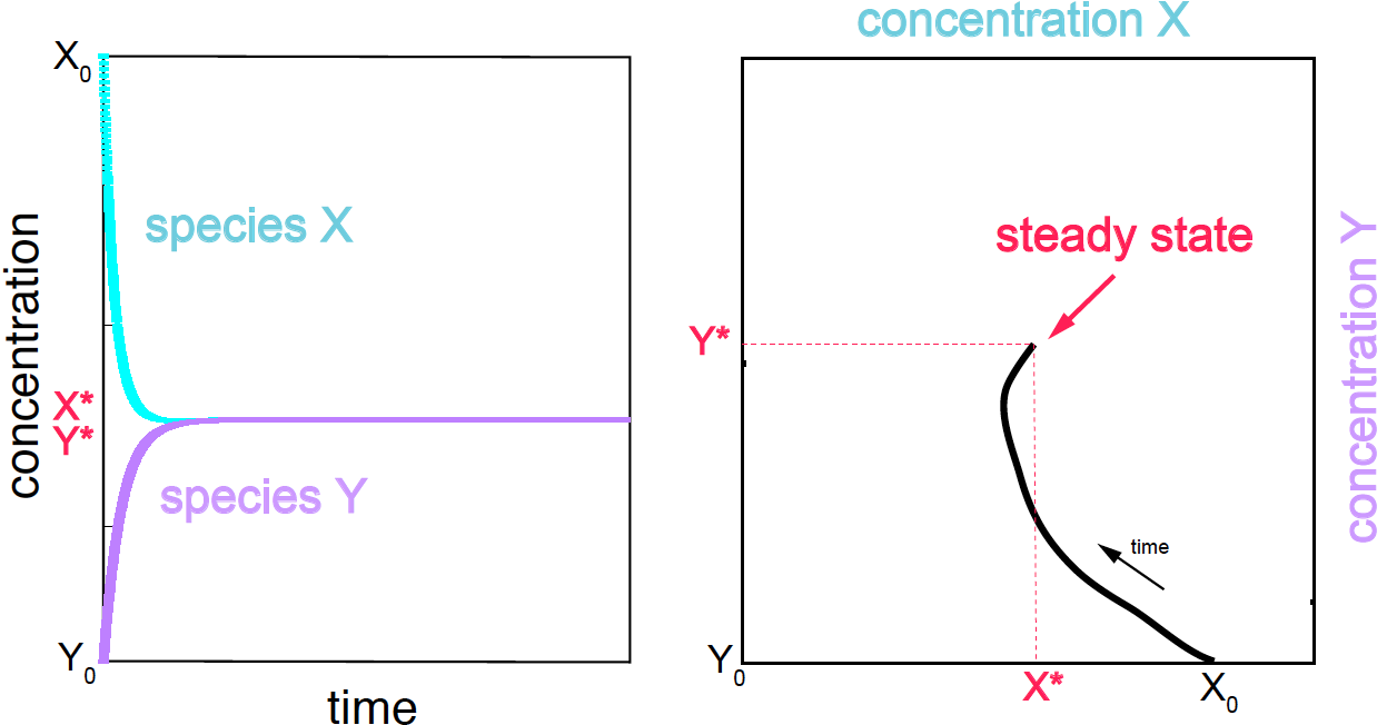
Figure 1. (A) Species concentration as a function of time. (B) Concentration trajectories in phase space.

The steady state

The steady state is defined as the value of the concentrations at which those would not further change as the reaction continues. That corresponds to the pair of species concentrations \(X^\ast\), \(Y^\ast\) such that

\[\begin{aligned} f_1(X^\ast,Y^\ast; k) &= 0\\ f_2(X^\ast,Y^\ast; k) &= 0\\ \end{aligned}\]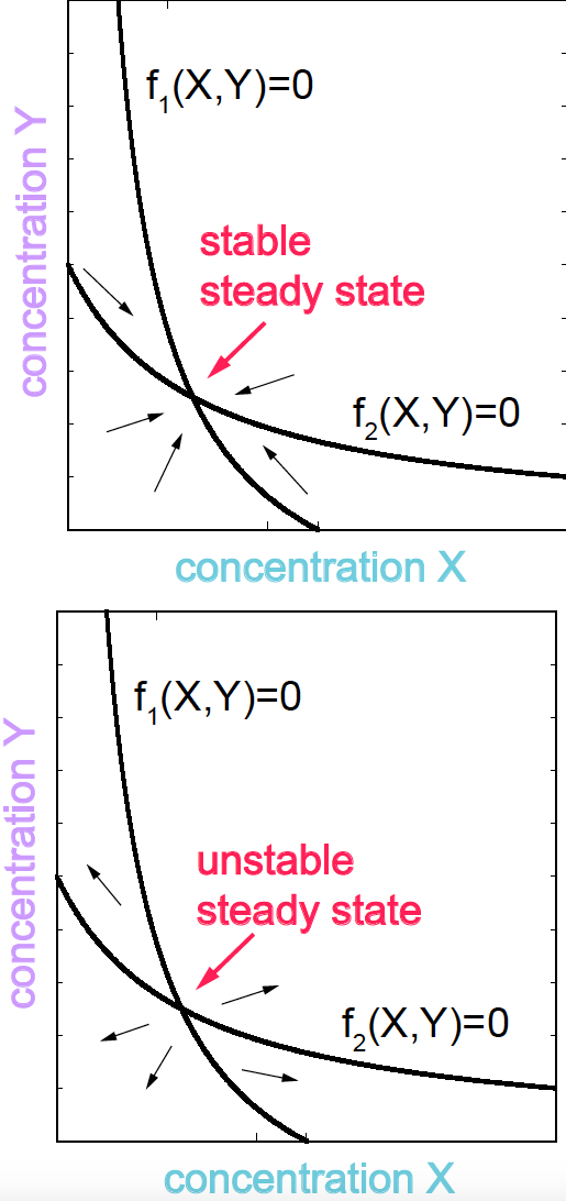

Figure 2. Nullclines.

If the initial conditions (\(X_0\) and \(Y_0\)) are different from the steady state values, the system will evolve (the concentrations of the species will change with time) until the steady state concentrations are reached, and the system does not evolve anymore.

But not all steady states are stable. In order to discuss that, let’s introduce the concept of phase-space.

Phase-space and Nullclines

One way of representing the system if by depicting the change of the concentration of each of the species involved in the reaction as a function of time (Figure 1 A). An alternative representation of the dynamics of a two-species system the system, is by depicting one concentration against the other as they change from a initial state \(X_0, Y_0\) to steady state \(X^\ast, Y^\ast\) (Figure 1B).

In the phase space, we can also depict the lines corresponding to the two independent conditions

\[\begin{aligned} f_1(X,Y; k) &= 0\\ f_2(X,Y; k) &= 0\\ \end{aligned}\]

These two lines are referred to as the nullclines. The points of intersection of the two nullclines determine the steady states of the system (Figure 2).

By calculating the values of \(f_1(X,Y;k)\) and \(f_2(X,Y;k)\) for different pair of values \((X,Y)\), around the nullclines it is possible to deduce the kinetics of the system, and whether a particular steady state point is stable or unstable (see Figure 2).

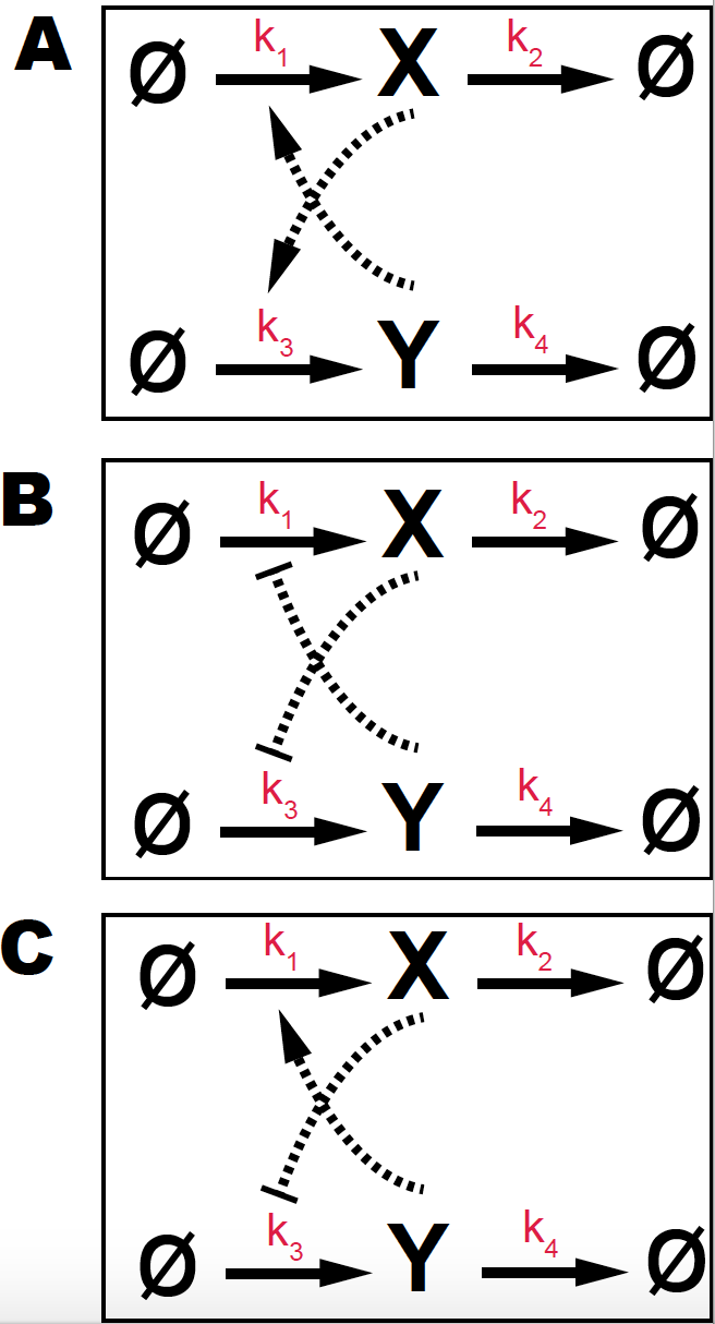
Figure 3. (A) Double positive feedback loop with two mutual activators (B) Double negative feedback loop with two mutual inhibitors. (C) Double positive/negative feedback loop with one activator and one inhibitor. Parameters are k1=k2=k3=k4 =1, and Hill coefficient K=0.5.

Double feedback loop regulatory networks

For the three reactions given in Figure 3 each with two feedback loops

Write the kinetic equations.
Draw several trajectories for different initial conditions for the two species.
Draw the nullclines in the phase space and indicate the direction of the trajectories starting from different initial conditions.
Identify the number of steady states and their nature (stable or unstable).
(for extra credit) For one of the three cases, sample the stochastic process using the Gillespie algorithm, and compare the results with those of the deterministic solution.

Compare all the above results for Hill coefficient \(n=1\) and \(n=4\).