MCB111: Mathematics in Biology (Fall 2024)
- p-value: definition
- Example:
- The Student’s t-test: a widely used p-value
- Correcting for multiple hypothesis testing
- Proper p-value etiquette
- Comparing p-values of different experiments – don’t
- And if you have more than one alternative hypothesis?
week 04:
Significance: The Student’s t-test and p-values
p-value: definition
You have a hypothesis \(H_1\), usually complicated, that you suspect may explain your experimental observations, and a null hypothesis \(H_0\), usually simpler, that could also explain your results.
A new result comes in for which you \(H_1\) hypothesis assigns a particular “score” \(= sc\).
The p-value of \(sc\) is the cumulative probability that using the null hypothesis you could have got that score or higher (assuming that higher score is better).
\[\mbox{pvalue}(sc) = P(\mbox{score} >= sc \mid H_0).\]If \(\mbox{p-value}(sc)\) is small, that means there is little chance of that score being obtained under the null model. A common mistake is to think that such a small p-value implies that your hypothesis \(H_1\) is true. A p-value says nothing about your hypothesis, but about the hypothesis you would like to reject. Rejecting the null hypothesis does not imply that your hypothesis is true.
Example:
Remember the homework where you where running a new experiment which for a previous researcher had a failure frequency of \(f^0= 0.2\), and you observed ‘ssfff’, that is, a sequence of 2 successes (s) followed by three failures (f) ?
We can introduce two hypotheses
-
\(H_0\): The failure frequency \(f\) is equal to \(f^0\) (\(f = 0.20\)).
-
\(H_1\): The failure frequency \(f\) is larger than \(f^0\) (\(f > 0.20\)).
The p-value approach
We can calculate what is the probability under the null hypothesis of obtaining in 5 attempts the observed result or something more extreme.
Those events are: ‘ssfff’, ‘sffff’, and ‘fffff’. Resulting in a p-value,
\[\begin{aligned} pval(\mbox{'ssfff'}) &= P(\mbox{'ssfff'}\mid H_0) +P(\mbox{'sffff'}\mid H_0) +P(\mbox{'fffff'}\mid H_0)\\ &= \frac{5!}{3!2!} 0.2^3 0.8^2 + \frac{5!}{4!1!} 0.2^4 0.8 + \frac{5!}{5!0!} 0.2^5 \\ &= 0.0512 + 0.0064 + 0.00032\\ &= 0.05792 \end{aligned}\]What would you do with this result?
Oftentimes, a p-value is used to “reject” the null hypothesis if the pvalue is smaller than \(0.05\). Would you or would you not reject the null hypothesis after this result? Why 0.05?
The Bayesian approach
We have learned to calculate the posterior probability \(P(f \mid \mbox{'ssfff'})\) which tell us a lot about the value of the failure parameter \(f\) given the data. Namely,
\begin{equation} P(f \mid \mbox{‘ssfff’}) = \frac{6!}{3! 2!}\, f^3 (1-f)^2, \end{equation}
which is given in Figure 1. The maximum of this posterior distribution is \(f^* = 0.6\), far away from the failure frequency \(f^0 = 0.2\) of the null hypothesis.
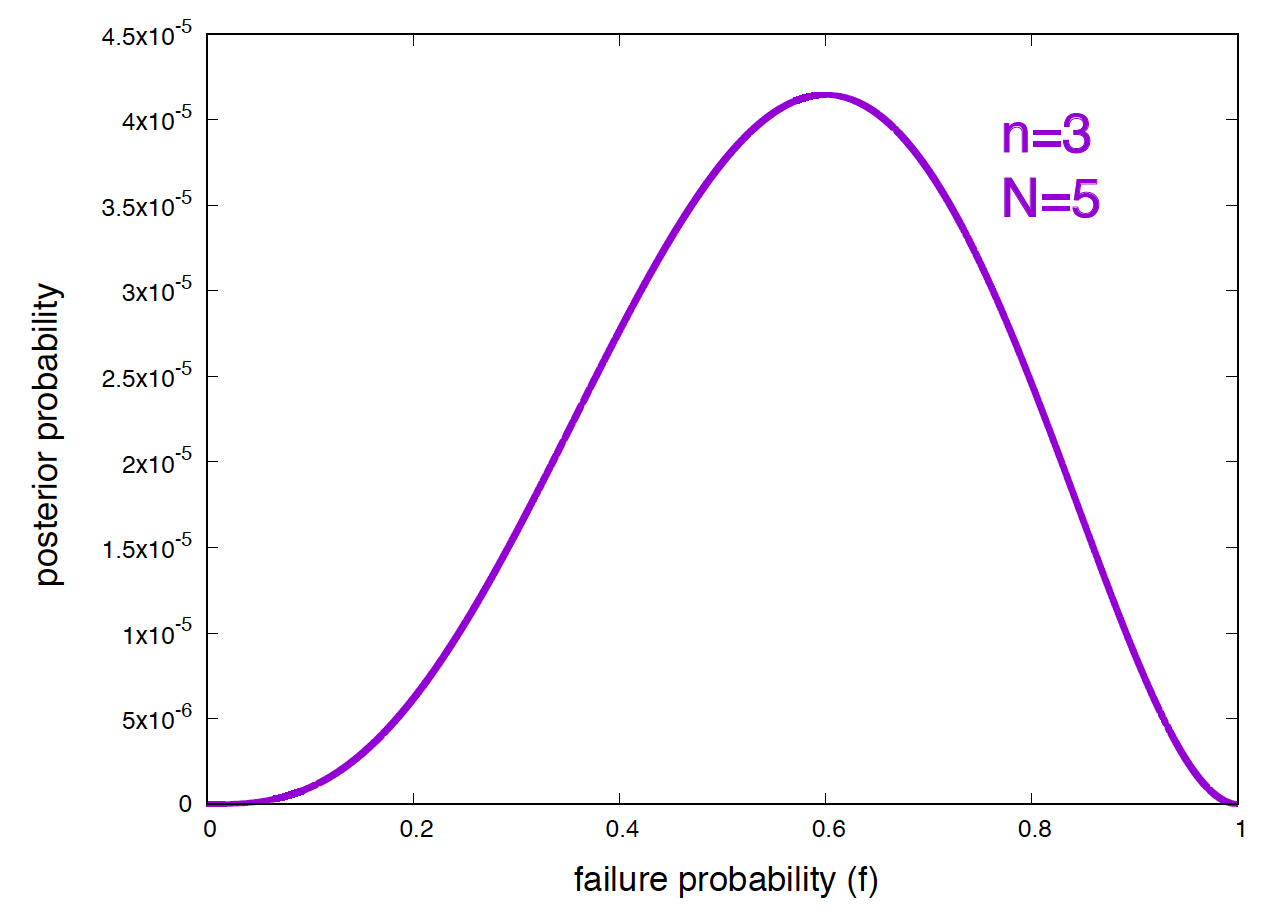
Figure 1. Posterior probabilities of the frequency of failure given that you have obtained 2 successes and 3 failures.
Bayesian hypothesis comparison tells us
\[\begin{aligned} \frac{P(H_0\mid \mbox{'ssfff'})}{P(H_1\mid \mbox{'ssfff'})} &= \frac{P(\mbox{'ssfff'}\mid H_0)\,P(H_0)} {P(\mbox{'ssfff'}\mid H_1)\,P(H_1)}. \end{aligned}\]Let us assume that both hypotheses are equally likely \(P(H_0) = P(H_1)\). Then the ratio of the two hypotheses is the ratio of the evidences of the data given \(H_0\) and \(H_1\), as
\[\begin{aligned} \frac{P(H_0\mid \mbox{'ssfff'})}{P(H_1\mid \mbox{'ssfff'})} &= \frac{P(\mbox{'ssfff'}\mid H_0)}{P(\mbox{'ssfff'}\mid H_1)}. \end{aligned}\]And using marginalization,
\[\begin{aligned} \frac{P(\mbox{'ssfff'}\mid H_0)}{P(\mbox{'ssfff'}\mid H_1)} &= \frac{\int_{0}^{1} P(\mbox{'ssfff'}\mid f, H_0)\,P(f\mid H_0)\, df} {\int_{0}^{1} P(\mbox{'ssfff'}\mid f, H_1)\,P(f\mid H_1)\, df}. \end{aligned}\]Let’s assume that for the \(H_0\) hypothesis the probability does not have to be precisely \(f^0\), but it can take the range \(f^0\pm 0.01\).
Using uniform priors
\[\begin{aligned} P(f\mid H_0) &= \left\{ \begin{array}{ll} \frac{1}{0.21-0.19} & \mbox{for}\quad 0.19 < f < 0.21\\ 0 & \mbox{otherwise} \end{array} \right.\\ P(f\mid H_1) &= \left\{ \begin{array}{ll} \frac{1}{1.0-0.2} & \mbox{for}\quad 0.2 < f < 1\\ 0 & \mbox{otherwise} \end{array} \right. \end{aligned}\]we have
\[\begin{aligned} \frac{P(H_0\mid \mbox{'ssfff'})}{P(H_1\mid \mbox{'ssfff'})} = \frac{P(\mbox{'ssfff'}\mid H_0)}{P(\mbox{'ssfff'}\mid H_1)} &= \frac{\int_{0}^{1} P(\mbox{'ssfff'}\mid f)\,P(f\mid H_0)\,df}{\int_{0}^{1} P(\mbox{'ssfff'}\mid f)\,P(f\mid H_1)\, df}\\ &= \frac{\frac{1}{0.02}\,\int_{0.19}^{0.21} f^3 (1-f)^2 \,df}{\frac{1}{0.80}\,\int_{0.2}^{1} f^3 (1-f)^2 \,df}\\ &= \frac{\frac{1}{0.02}\,\left[\frac{1}{4}f^4+\frac{1}{6}f^6-\frac{2}{5}f^5\right]^{0.21}_{0.19}} {\frac{1}{0.80}\,\left[\frac{1}{4}f^4+\frac{1}{6}f^6-\frac{2}{5}f^5\right]^{1}_{0.20}}\\ &= \frac{0.005127}{0.020480}\\ &= \frac{20.02}{79.98} \end{aligned}\]Thus, given the data and our priors, there is a 80:20 chance that the failure probability is larger than 0.2.
Which method do you prefer?
-
As you can see in this example, the p-value does not use any information about the \(H_1\) hypothesis, thus does not provide any information about \(H_1\), while the Bayesian method does.
-
Calculating a p-value can be easier, especially for methods with many parameters, and you should feel free to use it, provided that you know what you are doing, and interpret the results correctly. The above p-value of \(\sim\)0.06 does not mean that the probability of the null hypothesis being false is 94%, it is just the probability of obtaining the results you got under the null hypothesis.
Sometimes it is difficult to decide what to do with a given p-value result. More about this later in this lecture.
-
In my opinion, if possible, the Bayesian method is preferable as it conveys a lot more information. Just the posterior probability (Figure 1) gives you a lot of information about what the data tells about the value of the parameters. It is also more robust to small fluctuations as allowing you integrate around the value 0.2 for \(H_0\).
The Student’s t-test: a widely used p-value
It is typical to provide a p-value to compare the mean of a experimental distribution to a known mean of a null hypothesis. Let’s consider one practical case.
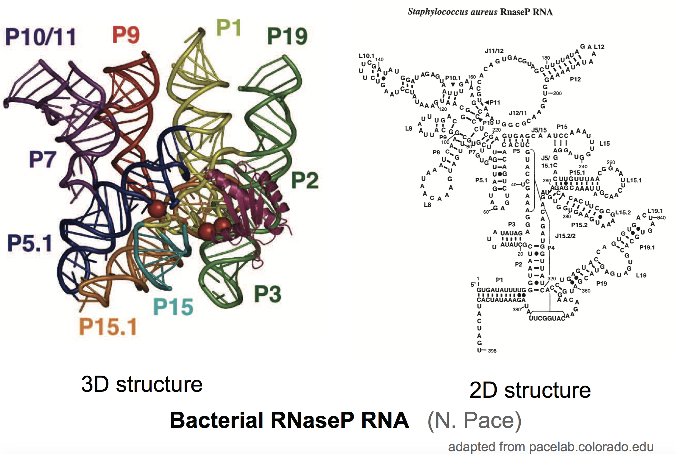
There are genes that do not produce proteins, but the functional product is the RNA molecule. Many of those functional RNAs form stable structures. RNaseP RNA is an example of a structural RNA that functions as a ribozyme (a RNA enzyme). RNaseP RNA is responsible for trimming the ends of tRNAs. As many other functional RNAs, RNAseP RNA has a structure.
Finding the structure of one of those functional RNAs is an interesting problem. One conclusive way is using crystallography, but that is hard and slow. We have faster computational methods that can predict structures given the RNA sequence. There are also experimental techniques (named RNA structural or chemical probing) that given an RNA molecule, can calculate the reactivity of each residue for rather long RNA molecules. These chemical reactivities correlate with the flexibility of the RNA molecule, thus they are expected to inform us about which residues are paired and unpaired in the molecule, thus providing experimental information about RNA structure (see for instance).
I have taken chemical probing data for a well known RNA molecule, RNaseP RNA, from the RNA Mapping DataBase ([RMDB])(https://rmdb.stanford.edu/), a repository of RNA structure probing. Here is the original data if you want to double check my analysis (which I encourage you to do). And here are the files extracted from the previous file of reactivities for bases that are paired, and reactivities for bases that are not paired, for the wild type RNaseP RNA sequence.
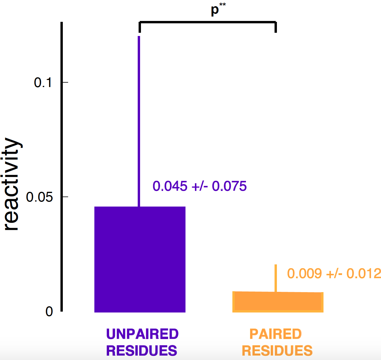
Figure 3. Mean and standard deviation for the reactivity data of one chemical probing experiment for RNaseP RNA.
In Figure 3, I show a typical plot. As you well know, I do not like those plots, and I think you should never use them. This plots simply tells us what the mean and standard deviation of the reactivities are if we separate the base paired residues from those that are unpaired.
Another typical thing to do is to add a mysterious p-value associated to that plot. I have followed that trend. Let the null hypothesis be that a residue is unpaired. One such typical method is called Student’s t-test. I have used a Python function that implements the Student’s t-test, named ttest_ind. I have used the ttest matlab function out of the box in order to calculate the p-value of the distribution of paired residues relative to that of unpaired residues (the null hypothesis).
The ttest function assigns a p-value of \(4.6e^{-9}\) for the paired residue distribution to have the mean of the unpaired residue distribution.
From this small p-value, you may be tempted to conclude that clearly you can use chemical probing data to distinguish between residues are paired from those that are not, thus to infer a structure for the RNA.
That conclusion would be wrong
Read the documentation – look at your data
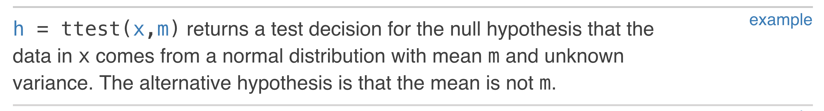
Figure 3. Matlab documentation for function ttest(x,m).
If you go to the matlab documentation for the ttest function, the first thing you read is that in order to use the Student’s t-test, the distribution of the data has to be Gaussian (see Figure 3). However, if you go to the Python documentation, they don’t even bother mentioning that fact. It is only when you go to the linked wikipedia pages.
Is that the case for this data?
Figure 4 shows that the distributions of reactivity scores both for paired and unpaired residues are obviously not Gaussian.
never use a p-value test without looking at the actual distribution first
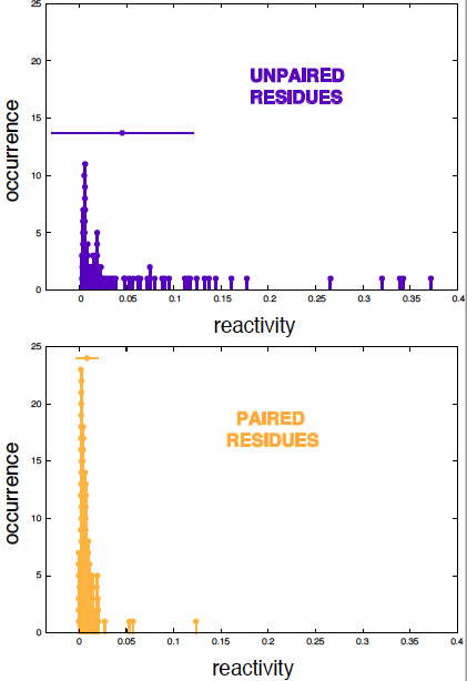
Figure 4. The distributions of reactivity scores for paired and unpaired residues.
What does the Student’s distribution have to do with any of this?
For this section, I am following Sivia’s book “Data Analysis”, Sections 2.3 and 3.2.
Let us be Bayesian again. We have an experiments in which the measurements \(\{x_k\}\) are Gaussian. The ttest calculates the probability that the experiment’s mean could have come from a process of mean \(\mu\).
Bayes’ theorem tells us that the posterior probability for the two parameters of the Gaussian distribution \(\mu\) and \(\sigma\) is given by
\[\begin{equation} P(\mu, \sigma\mid \{x_k\}, I) \propto P(\{x_k\}\mid \mu, \sigma, I) \times P(\mu, \sigma\mid I), \end{equation}\]where \(P(\mu, \sigma\mid I)\) is the prior probability of the parameters.
Since we are comparing only means, the Bayesian thing to do is to integrate to all possible values of the variance \(\sigma\)
\[\begin{equation} P(\mu\mid \{x_k\}, I) \propto \int_0^{\infty} P(\{x_k\}\mid \mu, \sigma, I) \times P(\mu, \sigma\mid I)\, d\sigma. \end{equation}\]The probability of the data given \(\mu\) and \(\sigma\) is
\[\begin{equation} P(\{x_k\}\mid \mu, \sigma, I) = \prod_k P(x_k\mid \mu, \sigma, I) = \frac{1}{\left(\sqrt{2\pi\sigma^2}\right)^N} \mbox{exp}\left[ -\frac{1}{2\sigma^2}\sum_{k=1}^N(x_k-\mu)^2\right]. \end{equation}\]Assuming uninformative and independent priors
\[P(\mu, \sigma\mid I) = P(\mu\mid I)\, P(\sigma\mid I)\]where
\[\begin{aligned} P(\mu\mid I) &= \left\{ \begin{array}{ll} \frac{1}{\mu_{+}-\mu_{-}} & \mbox{for}\quad \mu_{-} < \mu < \mu_{+}\\ 0 & \mbox{otherwise} \end{array} \right.\\ P(\sigma\mid I) &= \left\{ \begin{array}{ll} \mbox{constant} & \mbox{for}\quad \sigma > 0\\ 0 & \mbox{otherwise} \end{array} \right. \end{aligned}\]are constants, which allows us to include the prior in the proportionality.
The posterior probability of \(\mu\) is then
\[\begin{equation} P(\mu\mid \{x_k\}, I) \propto \int_0^{\infty} \frac{1}{\sigma^N} \mbox{exp}\left[ -\frac{1}{2\sigma^2}\sum_{k=1}^N(x_k-\mu)^2\right]\, d\sigma. \end{equation}\]Introducing a change of variable
\[t = \frac{\sqrt{\sum_k (x_k-\mu)^2}}{\sigma}\quad \mbox{then}\quad d\sigma = -\frac{\sqrt{\sum_k (x_k-\mu)^2}}{t^2}\, dt\]we obtain,
\[\begin{aligned} P(\mu\mid \{x_k\}, I) &\propto \int_0^{\infty} \left(\frac{t}{\sqrt{\sum_k (x_k-\mu)^2}}\right)^N \left(e^{-t^2/2}\right)\ \frac{\sqrt{\sum_k (x_k-\mu)^2}}{t^2}\, dt\\ &= \left(\sqrt{\sum_k (x_k-\mu)^2}\right)^{-N+1} \int_0^{\infty} t^{N-2} e^{-t^2/2} dt. \end{aligned}\]Then, since the integral is a constant that does not depend on the data or \(\mu\),
\[\begin{equation} P(\mu\mid \{x_k\}, I) \propto \left(\sum_k (x_k-\mu)^2\right)^{\frac{-N+1}{2}}. \end{equation}\]Introducing the sample mean \(\bar x = \frac{1}{N}\sum_k x_k\), and using the identity
\[\sum_k (x_k-\mu)^2 = N\left(\bar x - \mu\right)^2 + \sum_k\left(x_k-\bar x\right)^2,\]and introducing \(V\equiv \sum_k\left(x_k-\bar x\right)^2\) which is not dependent on \(\mu\)
we have,
\[\begin{equation} P(\mu\mid \{x_k\}, I) \propto \left[N (\bar x-\mu)^2 + V\right]^{\frac{-N+1}{2}}, \end{equation}\]which is one of many representations of the Student’s t distribution.
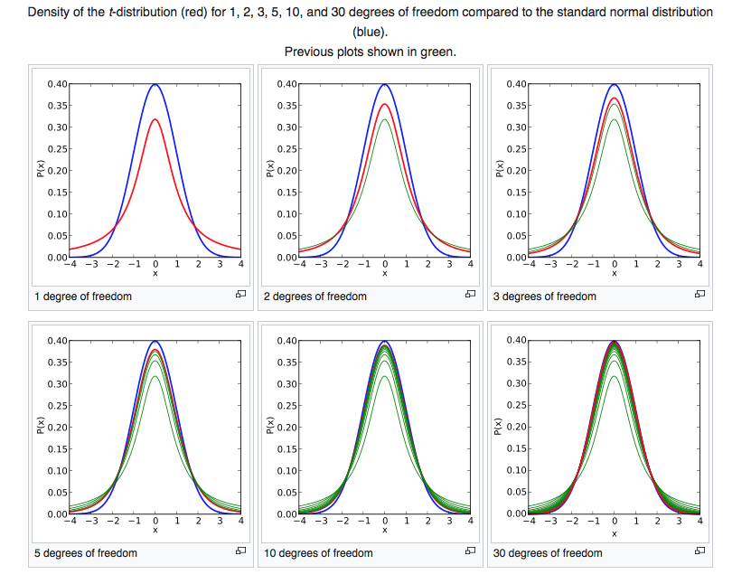
Figure 5. Comparison of the Student's t distribution for a zero sample mean and different values of N to the Gaussian distribution of mean zero and sigma one.
The Student’s distribution is much like the Gaussian distribution. It is symmetric around \(\mu\). The main difference from a Gaussian is that the tails are much fatter and they extend further from the mean value. As \(N\) becomes larger, the Student’s t distribution becomes closer to the Gaussian distribution. (See Figure 5).
Is this p-value what you really want to know?
Student’s t-test or not, it is obvious that the means of the two chemical probing distributions for paired and unpaired residues are different (Figure 4). For some experiments, knowing that the means are different is all you need. But let us think again about what we would like to achieve here. You want to see if chemical probing reactivities will help you distinguish residues that are base paired from those that are not paired.
The p-value calculation you would like to do is:
for a given reactivity value, what is the probability that I could have obtained that reactivity or smaller if the residue were unpaired?
We can calculate an empirical version of this p-value using the data we have. From the distribution of unpaired residues in Figure 4, I find
| reactivity | p-value | unpaired residues with this reactivity or lower |
|---|---|---|
| 0.0029 | 0.02 | 2% |
| 0.0034 | 0.05 | 5% |
| 0.0042 | 0.10 | 10% |
This results is telling us that we need to restrict to very small reactivities so that not too many false positives start appearing.
Notice that I have not had to invoke any fancy-named statistical test to do this calculation, nor have I had to make any assumptions about the data.
Remember that our objective is to decide on whether and how can I use the residue reactivities to infer which residues are paired and which aren’t. P-values refer to one single testing: I look at the reactivity of one single residue. Answering the above question requires testing all residues in the RNA structure. This is a problem of multiple testing that we approach next.
Correcting for multiple hypothesis testing
The p-values we have discussed so far give us a probability per test. If I do my experiment one more time, and I obtain one particular outcome, the p-value is the probability of that outcome (or another more extreme) happening just under the null hypothesis.
How to interpret a p-value if you repeat the experiment many times? This issue is very relevant in modern high-throughput biology. If you repeat a test many times, even a small p of obtaining that result under the null hypothesis, could results in a large number of cases controlled by the null hypothesis with p-value \(p\) or smaller (false positives).
How many false positives? approximately \(n p\), for \(n\) tests, when you assume that all observed scores come from the null hypothesis.
Here is a good read about what to do with p-values for multiple testing “How does multiple testing correction work?” by W. Noble
The bonferroni correction: controlling the familywise error rate
A simple thing to do is, if you aim for a certain p-value \(p\) and you do \(n\) tests, impose that for any given test you obtain a p-value of p/n. This is called the bonferroni correction.
This is also called controlling the familywise error rate, as \begin{equation} P(\cup_i {p_i \leq p}) \leq \sum_i P(p_i\leq p/n) \leq n \frac{p}{n} = p. \end{equation}
This is considered a very conservative approach for very large number or tests.
False Discovery Rate (FDR)
Let’s go back to our problem of using chemical probing data to estimate RNA residues that are paired into a structure.
-
N = number of tests (number of residues in the RNA molecule, N=265)
-
\(sc^\ast\) a chosen score (reactivity)
-
\(p^\ast\) p-value probability that a unpaired residue has a score \(sc \leq sc^\ast\).
-
\(F^\ast\) number of residues with a score \(sc \leq sc^\ast\).
The False Discovery Rate is defined as the fraction of the measurements we called positives at the p-value threshold \(p^\ast\) (named above \(F^\ast\)), that are expected to be false positives. That is, assuming that all \(N\) measurements are drawn from the null hypothesis,
\[\begin{aligned} \mbox{FDR} &= \frac{\mbox{N} \times p^\ast}{F^\ast}. \end{aligned}\]Introducing also
-
\(T\) = Trues (residues that are paired, N=160)
-
\(TF^\ast\) = number of T with a score \(sc \leq sc^\ast\), that is, T \(\cap\, F^\ast\).
We can calculate the sensitivity corresponding to that FDR as
\[\begin{aligned} \mbox{Sensitivity} &= \frac{TF^\ast}{T}. \end{aligned}\]In a given experiment, you want to find a good tradeoff between the cost of having false positive (the FDR) with the benefit of finding more positives (the sensitivity).
Using the data we have, we can calculate p-values, FDR, and sensitivity for different reactivity scores as,
| reactivity | p-value | FDR | Sensitivity (%) |
|---|---|---|---|
| 0.0029 | 0.02 | 0.17 | 17 |
| 0.0034 | 0.06 | 0.34 | 24 |
| 0.0042 | 0.10 | 0.45 | 33 |
| 0.0063 | 0.28 | 0.67 | 50 |
Thus, in order to identify 50% of the paired bases (sensitivity), you should expect that about 66% of the bases that you call paired are really not paired (FDR). This is a more informative and sober view of the power of chemical probing, than our original assertion about the means of the two distribution being different with a very small p-value.
Proper p-value etiquette
As David Mackay puts it, “[..] p-values [..] should be treated with extreme caution”. Even the American Statistical Association has issued recent warnings on the use of p-values
What p-values are not
-
p-values say nothing about your beloved hypothesis. Rejecting the null hypothesis does not mean that your hypothesis is true.
-
p-values are not the probability of the null model given the data. p-values tell you about the probability of the data, given the null hypothesis. A p-value of 0.01 does not mean that there is a 1% chance for the null model to be true; rather, that you should expect a 1% false positives.
-
p-values are not posteriors of the null model given the data, and cannot be used to asses model strength or to compare different models.
-
p-values are often used as a measure of statistical significance, but that is bogus. p-values tell you about the number of false positives that have sneaked into your experiment. In an experiment with \(N\) observation, a p-value of \(p\) means that you should expect find about \(N p\) false positives amongst your positives.
-
Is a small p-value significant? Remember from our w01 lectures, the \(CDF_X(X)\) is distributed uniformly. Thus, a p-value which are values from a CDF is also distributed uniformly.
If your data follows the null hypothesis, you should be as surprised of getting a p-value of 0.05 as you would be of getting a 0.99 or any other value, because they are being drawn from a Uniform \([0.1]\) distribution.
Define precisely your p-value as a probability of something
When you say you are calculating a p-value, you cannot assume the reader should know what you are talking about. And conversely, if you read in a paper that something is “significant with a p-value of blah” and that is all the explanation they provide, do not feel stupid if you have no idea what they are talking about!
Specify the null hypothesis
It is also not obvious what the null hypothesis is, that should always be specified.
Look in your data for those expected false cases
Do not use the word “significant”. All a p-value is giving you is an idea of how many false positives you should find in your set of predictions. It is your responsibility to estimate if that number is reasonable or not, and to find those false predictions. They may give you an idea of other effects (alternative hypotheses) that you are so far ignoring.
Comparing p-values of different experiments – don’t
There is an infectious disease that if left untreated, affected people have a probability of recovery of \(p_0 = 0.4\). We will call this the null hypothesis \(H_0\).
Your lab is testing two new treatments, treatment A (TrA) and treatment B (TrB). You run two different experiments (expA and expB) where TrA or TrB is given to two different groups of affected people.
Your analysis tells you that the p-values for the outcomes of expA and expB respect to the null hypothesis \(H_0\) are
\[\begin{aligned} \mbox{pval}(expA) &= 0.2131,\\ \mbox{pval}(expB) &= 1.05 e^{-5}.\\ \end{aligned}\]It seems tempting to conclude from this results that TrB is a more effective treatment than TrA.
That conclusion would be wrong.
You can never compare two hypotheses by looking to their p-values relative to a third null hypothesis. There are many hidden and possibly confounding variables in that calculation, one of them the sample size.
Let’s see what could be going on behind the scenes. A way of obtaining the previous result is the following:
- expA includes 15 infected people, 8 of which recovered after using TrA.
- expB includes 300 infected people, 157 of which recovered after using TrB.
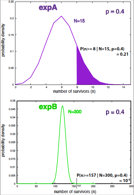
Figure 6. Probability density under the null hypothesis and p-values for expA and expB.
The corresponding p-values, that is, the probabilities of at least 8 (157) recoveries out of 15 (300) under the null hypothesis \(H_0\) of no treatment at all are
\[\begin{aligned} \mbox{pval}(expA) &= \sum_{n=8}^{15} P(n\mid N=15, p_0) \\ &= \sum_{n=8}^{15} \frac{15!} {n! (15-n)!} 0.4^n 0.6^{15-n} \\ &= 0.2131,\\ \mbox{pval}(expB) &= \sum_{n=157}^{300} P(n\mid N=300, p_0) \\ &= \sum_{n=157}^{300} \frac{300!}{n! (300-n)!} 0.4^n 0.6^{300-n} \\ &= 1.05 e^{-5}.\\ \end{aligned}\]However, any simple analysis (for instance looking at the sample mean for \(p_A\) and \(p_B\), the probabilities of survival under TrA and TrB) tell you that those two treatments seem to be similar in effectiveness,
\[\begin{aligned} p_A^* &= \frac{8}{15} = 0.533,\\ p_B^* &= \frac{157}{300} = 0.523. \end{aligned}\]What is going on?
Because the sample sizes for the two experiments are so different, the distribution \(P(n\mid N=300, H_0)\) is much narrower than \(P(n\mid N=15, H_0)\), thus the p-value of expB is smaller simply because the sample size is larger (see Figure 6).
If you calculate the posterior distributions \(P(p_A\mid expA)\) and \(P(p_B\mid expB)\), which we have done before in w02,
\[\begin{aligned} P(p_A\mid expA) &= \frac{16!} {8! 7!}\, p_A^{8} (1-p_A)^{7}\\ P(p_B\mid expB) &= \frac{301!}{157! 143!}\, p_B^{157} (1-p_B)^{143} \\ \end{aligned}\]you can conclude that your assessment of \(p_B\) is more precise than that of \(p_A\), due to the larger amount of data, but they are perfectly compatible with both treatments having the same effectiveness. (see Figure 7).
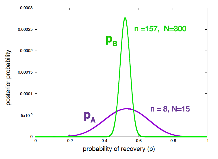
Figure 7. Posterior probability of the efficiency of treatment A and treatment B given the data.
As we did in the homework of w02, you remember that when the data follows a binomial distribution, the best estimate of the Bernoulli parameter \(p\) and its confidence value are given by
\[\begin{equation} p^\ast = \frac{n}{N} \quad \sigma = \sqrt{\frac{p^\ast(1-p^\ast)}{N}}. \end{equation}\]The best estimates and confidence values for the effectiveness of the two treatments are
\[\begin{aligned} p_A &\approx 0.533 \pm 0.129\\ p_B &\approx 0.523 \pm 0.029. \end{aligned}\]In fact, if the two experiments had been run with using the same treatment, you would have obtained one “significant” p-value and one “non significant” p-value just because of the different sample size.
In each case, the p-value is telling you the right thing regarding the null hypothesis. For expA, you don’t have enough data to reject \(p_A=p_0=0.4\), which is the same than the posterior of \(p_A\) in Figure 7 is telling you. On the other hand, for expB, you have enough data to reject \(p_B=p_0=0.4\) as a likely value of the probability of recovery. The wrong statement is to use those two results to make any claims about the effectiveness of TrA versus TrB. The posterior distributions of \(p_A\) and \(p_B\) in Figure 7 are telling you a lot more (with the same data) regarding the likelihood of any possible value of the probability of recovery under each treatment.
And if you have more than one alternative hypothesis?
The Bayesian approach to the question of comparing multiple hypothesis is clear. If you had multiple hypotheses \(H_1\ldots H_n\), one can calculate
\[P(H_i\mid D) = \frac{P(D\mid H_i)\ P(H_i) } {P(D\mid H_1)\ P(H_1) + \ldots + P(D\mid H_n)\ P(H_n)}, \quad 1\leq i \leq n,\]which just requires to specify some priors for the different hypotheses.
I am not sure how to come up with a p-value-based calculation using more than one null hypothesis.