MCB111: Mathematics in Biology (Fall 2024)
week 06:
Probabilistic models and Inference
In this week’s lectures, we discuss probabilistic graphical models and how to do inference using them. As a practical case, we are going to implement the probabilistic model introduced by Andolfatto et al. to assign ancestry to chromosomal segments.
There are many good books to learn about probabilistic models. “Probabilistic graphical models: principles and techniques” (by Koller & Friedman) is a comprehensive source about more general probabilistic models than the one we are going to study here. “Biological sequence analysis” (by Durbin et al.) while concentrates on genomic sequences, is a good reference to learn about some basic (and widely used) probabilistic models, as it provides detailed descriptions of some of the fundamental algorithms. Another good source is “Pattern Theory” (by Mumford and Desolneux).
Probabilistic Graphical Models
Definition
A probabilistic graphical model is a graphical representation of the relationships between different random variables. It consists of nodes that represent random variables and edges that represent their relationships by conditional probabilities. Probabilistic graphical models also go by the name of Bayesian networks (BN).
Let me light it up with an example in Figure 1 taken from Koller & Friedman.
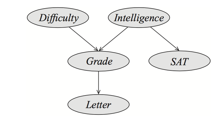
Figure 1. A example of a Bayesian network (BN).
A professor is writing a recommendation letter for a student. Let’s “letter” be the strength of the letter. The strength of the letter is going to be based on the student’s “grades”, and “SAT” scores, both of which are available to the professor. The model in Figure 1 assumes that the grades depend both on the student’s “intelligence”, and on the course’s “difficulty”, while the “SAT” scores depend only on the intelligence.
The parts of the Bayesian network
The random variables are
- intelligence (\(i\))
- course difficulty (\(d\))
- course grades (\(g\))
- SAT scores (\(s\))
- strength of letter (\(l\))
Thus, we have a joint distribution of 5 random variables
\[P(d,i,g,s,l)\]With all generality (using the chain rule) we can write
\[\begin{aligned} P(d, i, g, s, l) &= P(l\mid d,i,g,s)\, P(d,i,g,s)\\ &= P(l\mid d,i,g,s)\, P(s\mid d,i,g)\, P(d,i,g)\\ &= P(l\mid d,i,g,s)\, P(s\mid d,i,g)\, P(g\mid d,i)\, P(d,i)\\ &= P(l\mid d,i,g,s)\, P(s\mid i) \, P(g\mid d,i)\, P(i\mid d)\, P(d)\\ \end{aligned}\]This is a complex set of possible dependencies, some of which do not really exist for the problem at hand; for instance, the intelligence of the student is not dependent of the difficulty of the courses she takes, thus in the expression above \(P(i\mid d) = P(i)\).
What the BN in Figure 1 describes is how to simplify the joint distribution of the 5 random variables. It is telling us which are the dependencies (amongst all possible) that we are going to consider. The edges represent conditional dependences between the random variables (nodes), such that the node at the end of the arrow depends on the node from where the edge starts. In a general BN, a node can have many arrows landing on it (many dependencies) from other nodes.
The graphical model in Figure 1 says that
\[\begin{aligned} P(l\mid d,i,g,s) &= P(l\mid g)\quad \mbox{"l" does not directly depend on "d", "i", or "s"} \\ P(s\mid d,i,g) &=P(s\mid i)\quad \mbox{"s" does not directly depend on "d", or "g"} \\ P(i\mid g) &=P(i)\quad \mbox{"i" does not directly depend on "g"} \\ \end{aligned}\]so that, the joint probability of all random variables is given by
\[P(d,i,g,s,l) = P(l\mid g)\, P(s\mid i)\, P(g\mid d,i)\, P(i)\, P(d).\]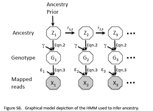
What to do with a Bayesian network?
Inference. Inference about some of the random variables, assuming that we have information about others.
In a Bayesian network, the random variables for which we have information become the evidence. From the other variables, we can decide which to do inference on and which to treat as hidden variables which will be integrated out to all possible values in order to make our inferences.
Several scenarios for the student letter example,
-
We know the outcome of “letters”, and also have access to the grades and SAT scores, and we may want to infer the intelligence of the student.
In this case the course grades will become a “hidden” variable that you will integrate out to all values.
-
You want to predict the strength of the letter you will be able to write by knowing the grades and SAT scores, in which case both intelligence and course difficulty become hidden variables.
Let’s approach inference with a probabilistic graphical model using a biology example implemented recently.
Our example: From genomic reads to recombination breakpoints
The probabilistic model proposed by Andolfatto et al. is given in their Figure S8 reproduced here. The problem is to assign ancestry (homozygous for one of the parents or heterozygous) to the different genomic loci of a given male fly by analyzing genomic reads.
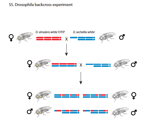
Andolfatto uses males flies created by crossing female F1 hybrids of Drosophila Simulans (Dsim) and Drosophila Sechellia (Dsec) with Dsec males. The resulting males would have an ancestry (Z) that is either Dsec/Dsec or Dsec/Dsim at different loci (see Figure S5 from Andolfatto et al. reproduced here). The genotype (G), that is the collection of actual nucleotides in both alleles, is unknown, and will be treated as a nuisance variable. What we know from the experiment is a collection of mapped reads (X) for each locus (genomic position).
For a given locus in one individual, the question is how to determine which reads correspond to parent Dsim versus parent Dsec, which will in turn determine the ancestry (Z) of the locus being either \(Dsim/Dsec\) or \(Dsec/Dsec\). Because the F1 females were crossed only to parent \(Dsec\) males (but not to parent \(Dsim\) males), the genotype \(Dsim/Dsim\) does not occur. (The reason for only crossing F1 females is because the F1 males are sterile.)
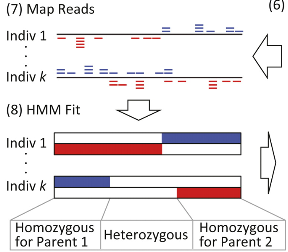
Figure 1 from Andolfatto et al. (http://genome.cshlp.org/content/21/4/610.full)
Andolfatto’s model assumes a more general situation in which the ancestry of a given individual at different loci, named \(Z\), could be either AA, or BB, or AB (Figure 1 from Andolfatto et al. reproduced here).
The Model (a Hidden Markov Model)
The random variables
Figure 2 shows an example of the three random variables for the problem of inferring ancestry from mapped reads with specific examples.
The random variables for a given locus (i.e. a genomic position) \(i\) are
-
\(X_i\) is the collection of reads for locus \(i\).
\[X_i = \{n^i_a, n^i_c, n^i_g, n^i_t\},\]where \(n^i_a\) is the number of read that have residue “a” at the locus \(i\)
-
\(G_i\) is the genotype at locus \(i\)
\[G_i \in \{aa, ac, ag, at, cc, cg, ct, gg, gt, tt \},\]are the actual residues at the locus for the two alleles. We have no information about order, thus there are 10 possible values for \(G_i\).
-
\(Z_i\) is the ancestry at locus \(i\)
\[Z_i \in \{AA, BB, AB\}\]where \(AA\) means the locus is homozygous for parent \(A\), \(BB\) means the locus is homozygous for parent \(B\), and \(AB\) means the locus is heterozygous.
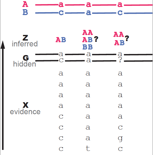
Figure 2. An illustration of problem of inferring ancestry from mapped reads. Three loci are given as examples.In principle, each \(Z_i\) can take three values. For the particular experiment described by Andolfatto et al. (assigning \(A = Dsim\) and \(B= Dsec\)), only two cases are possible \(BB\) and \(AB\), as the backcrosses are between Dsim/Dsec females and Dsec/Dsec males (Figure S5). Andolfatto describes the more general model with three possible ancestors.
The conditional probabilities
We want to calculate the joint probability of all random variables for all sites \(1\leq i \leq L\), for a chromosome of length \(L\),
\[P(X_1 G_1 Z_1,\ldots, X_L G_L Z_L).\]The Bayesian network in Andolfatto’s Figure S8, establishes the following dependencies
\[P(X_1 G_1 Z_1 \ldots X_L G_L Z_L) = P(X_1 G_1 Z_1)\ P(X_2 G_2 Z_2 \mid X_1 G_1 Z_1)\ \ldots P(X_{L} G_{L} Z_{L} \mid X_{L-1} G_{L-1} Z_{L-1}).\]This particular set of dependencies in the joint probability such that the probabilities at one node \(i\) depends only on the probability at the node before \(i-1\), define this model as a Hidden Markov Model. Hidden Markov Models (HMMs) are a subset of of the much larger set of probabilistic graphical models or Bayesian networks.
This graphical model also tells us (see Figure S8)
\[\begin{aligned} P(X_i G_i Z_i \mid X_{i-1} G_{i-1} Z_{i-1}) &= P(Z_{i}\mid Z_{i-1}) \, P(G_{i}\mid Z_{i})\, P(X_{i}\mid G_{i}),\\ P(X_1 G_1 Z_1) &= P_{\mbox{prior}}(Z_{1}) \, P(G_{1}\mid Z_{1})\, P(X_{1}\mid G_{1}).\\ \end{aligned}\]The inference question
An example of the inference problem is given in Figure 2. Figure 2 shows three loci as examples. Each locus has 8 mapped reads (the evidence). We also know the genome sequence of the two parental species A (top in red) and B (top in blue). The data for the first locus almost unambiguously indicates that the ancestry is AB. For the two other loci, either due to ambiguity or errors in the reads both possibilities AB and BB are plausible. The question is which one is the more likely?
We know the reads \(\{X_i\}_1^L\), and we want to infer the ancestry for each locus \(\{Z_i\}_1^L\). Thus, the \(\{G_i\}_1^L\) are hidden random variables that we want to integrate.
The joint marginal is given by
\[P(X_1 Z_1,\ldots, X_LZ_L) = \sum_{G_1} \ldots \sum_{G_L} P(X_1 G_1 Z_1,\ldots, X_L G_L Z_L).\]Because of the Markovian nature of this particular Bayesian network
\[\begin{aligned} P(X_1 Z_1,\ldots, X_LZ_L) &= \prod_{i} P(Z_i\mid Z_{i-1}) \sum_{G_i} P(G_{i}\mid Z_{i})P(X_{i}\mid G_{i}) \\ &= \prod_{i} P(Z_i\mid Z_{i-1})\,P(X_{i}\mid Z_{i}) \end{aligned}\]for the marginal probabilities are
\[P(X_{i}\mid Z_{i}) \equiv \sum_{G_i} P(G_{i}\mid Z_{i})\, P(X_{i}\mid G_{i}).\]The parameters
The conditional probabilities of this probabilistic model can be separated into two depending on whether they are conditioned on the locus before or not:
-
The \(P(Z_i\mid Z_{i-1})\).
Because any ancestry \(Z\) can be one of three cases \(Z=\{AA, BB, AB\}\), those represent three conditional probability distributions \(P(Z\mid AA)\), \(P(Z\mid BB)\), \(P(Z\mid AB)\).
given by
\[\begin{aligned} &P(AA\mid AA) \quad P(BB\mid BB) \quad \\ &P(AB\mid AA) \quad P(AB\mid BB) \quad a\ breakpoint\\ &P(BB\mid AA) \quad P(AA\mid BB) \quad a\ double\ breakpoint\\ \end{aligned}\]and
\[\begin{aligned} &P(AB\mid AB) \\ &P(AA\mid AB) \quad a\ breakpoint\\ &P(BB\mid AB) \quad a\ breakpoint\\ \end{aligned}\] -
The \(P(X_i\mid Z_{i})\).
More about these probability distributions when we get to the homework.
Figure 3 shows a different graphical representation of the Andolfatto HMM, where all the parameters that connect one locus with the next are explicit.
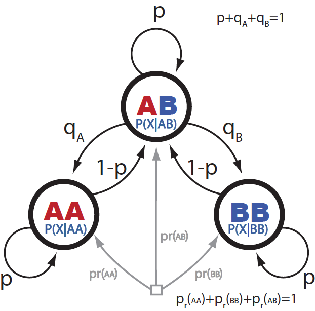
Figure 3. Graphical representation of the HMM for assigning ancestry.
Andolfatto et al., sets these parameters by looking at actual data.
Double breakpoints are not observed,
\[P(AA\mid BB) = 0\\ P(BB\mid AA) = 0.\]If we assume that all segment have on average the same length then we can use one single parameter to characterize when there is no breakpoint as
\[P(AA\mid AA) = P(BB\mid BB) = P(AB\mid AB) = p.\]Finally, Andolfatto uses the fact that on average there is about 1 breakpoint per chromosome in Drosophila species. The length of a region without breakpoints is determined by a geometric distribution of Bernoulli parameter \(p\)
\[l = \frac{p}{1-p}.\]Then having on average only two regions (one breakpoint) per chromosome of length \(L\), results in
\[\frac{L}{2} = \frac{p}{1-p}.\]or
\[p = \frac{L}{L+2},\]for a chromosome of length \(L\).
Next week’s lectures will cover parameter estimation for a probabilistic model.
Inference
Using the probabilistic model (Figure1 and Andolfatto’s Figure S8) we can do calculate the breakpoints for a given chromosome of a given individual. In order to do that, we need to calculate the probability of the mapped reads under any possible ancestry
\[P(X_1 \ldots X_L) = \sum_{Z_1}\ldots\sum_{Z_L} P(X_1 Z_1,\ldots, X_LZ_L).\]We will see later why we need to calculate this quantity. Let’s focus know on how are we going to calculate it.
Because of the Markovian property of this particular probabilistic model, we can write
\[P(X_1 \ldots X_L) = \sum_{Z_1}\ldots\sum_{Z_L} P(X_1 Z_1)\ P(X_2 Z_2\mid X_1 Z_1)\ldots P(X_L Z_L\mid X_{L-1} Z_{L-1}).\]This marginal probability has \(3^L\) terms, too many in general to be calculated directly.
Fortunately, we can calculate that marginal probability very efficiently with an algorithm that is linear in \(L\) instead of exponential.
In fact, we have two algorithms that can calculate \(\) efficiently, the forward and backward algorithms. We are introducing both, because both algorithm will be used to infer the breakpoints.
Forward Algorithm
For each locus \(1\leq i\leq L\), we define \(f_{Z}(i)\) as the probability of loci \(X_1\ldots X_{i}\), where all loci from \(1\ldots i-1\) have been marginalized (sumed) to all possible ancestry, and loci \(i\) has ancestor \(Z\), that is
\[\begin{aligned} f_{Z}(i) &= P(X_1\ldots X_{i-1}, X_{i} Z_i=Z)\\ &= \sum_{Z_1}\ldots\sum_{Z_{i-1}} P(X_1 Z_1\ldots X_{i-1} Z_{i-1}, X_{i} Z_i=Z)\\ &= \sum_{Z_1}\ldots\sum_{Z_{i-1}} P(X_1 Z_1)\ P(X_2 Z_2\mid X_1 Z_1)\ldots P(X_{i-1} Z_{i-1}\mid X_{i-2} Z_{i-2})\ P(X_i Z_i=Z\mid X_{i-1} Z_{i-1})\\ &= \sum_{Z_{i-1}} P(X_i Z_i=Z\mid Z_{i-1})\ f_{Z_{i-1}}(i-1). \end{aligned}\]The name forward should be self-explanatory now. In order to calculate \(f_Z(i)\), I need to know \(f_{Z}(i-1)\), …
More explicitly, the forward probabilities are calculated using a forward recursion starting from \(i = 2\)
\[\begin{aligned} f_{AA}(i) = P(X_i\mid AA)\ [ &+ p \, f_{AA}(i-1) \\ &+ q_A\, f_{AB}(i-1)] \\ f_{BB}(i) = P(X_i\mid BB)\ [ &+ p \, f_{BB}(i-1) \\ &+ q_B\, f_{AB}(i-1)] \\ f_{AB}(i) = P(X_i\mid AB)\ [ &+ p \, f_{AB}(i-1) \\ &+ (1-p)\, f_{AA}(i-1) \\ &+ (1-p)\, f_{BB}(i-1)] . \end{aligned}\]The initialization conditions for \(i=1\) use the prior probabilities \(P(X)\). For the first locus,
\[\begin{aligned} f_{AA}(1) &= P(X_1\mid AA)\, P(AA) \\ f_{BB}(1) &= P(X_1\mid BB)\, P(BB) \\ f_{AB}(1) &= P(X_1\mid AB)\, P(AB) \\ \end{aligned}\]Then the probability \(P(X_1\ldots X_L)\) is given by
\[P(X_1\ldots X_L) = f_{AA}(L) + f_{BB}(L) + f_{AB}(L).\]This type of algorithm is called a dynamic programming (DP) algorithm. Dynamic programming algorithms were introduced by Richard Bellman in 1954.
Backward Algorithm
For each locus \(1\leq i\leq L\), we define \(b_{Z}(i)\) as the probability of \(X_{i+1}\ldots X_{L}\) (summing to all possible ancestry), conditioned on the fact that locus \(i\) has ancestor \(Z \in \{AA, BB, AB\}\).
\[\begin{aligned} b_{Z}(i) &= P(X_{i+1}\ldots X_L\mid Z_i=Z)\\ &= \sum_{Z_{i+1}}\ldots\sum_{Z_{L}} P(X_{i+1} Z_{i+1}\ldots X_L Z_L\mid Z_i=Z)\\ &= \sum_{Z_{i+1}}\ldots\sum_{Z_{L}} P(X_{i+1}Z_{i+1}\mid Z_i = Z)\ P(X_{i+2} Z_{i+2}\mid X_{i+1} Z_{i+1})\ \ldots P(X_{L-1} Z_{L-1}\mid X_{L-2} Z_{L-2})\ P(X_L Z_L\mid X_{L-1} Z_{L-1})\\ &=\sum_{Z_{i+1}} P(X_{i+1}Z_{i+1}\mid Z_i = Z)\ b_{Z_{i+1}}(i+1). \end{aligned}\]The name backward should be self-explanatory now. In order to calculate \(b_Z(i)\), I need to know \(b_{Z}(i+1)\), …
Those backward probabilities are calculated using a backwards recursion starting from \(i = L-1\)
\[\begin{aligned} b_{AA}(i) &= \begin{array}{r} + p \, b_{AA}(i+1)\, P(X_{i+1}\mid AA)\\ + (1-p)\, b_{AB}(i+1)\, P(X_{i+1}\mid AB) \end{array} \\\\ b_{BB}(i) &= \begin{array}{r} + p \, b_{BB}(i+1)\, P(X_{i+1}\mid BB)\\ + (1-p)\, b_{AB}(i+1)\, P(X_{i+1}\mid AB) \end{array} \\\\ b_{AB}(i) &= \begin{array}{r} + p \, b_{AB}(i+1)\, P(X_{i+1}\mid AB)\\ + q_A \, b_{AA}(i+1)\, P(X_{i+1}\mid AA)\\ + q_B \, b_{BB}(i+1)\, P(X_{i+1}\mid BB) \end{array} \end{aligned}\]The initialization conditions for \(i=L\) use the prior probabilities \(P(X)\)
\[\begin{aligned} b_{AA}(L) &= 1, \\ b_{BB}(L) &= 1, \\ b_{AB}(L) &= 1. \\ \end{aligned}\]The backward probabilities are calculated independently from the forward probabilities.
The probability \(P(X_1\ldots X_L)\) is given by
\[P(X_1\ldots X_L) = f_{AA}(1)\ b_{AA}(1) + f_{BB}(1)\ b_{BB}(1) + f_{AB}(1)\ b_{AB}(1).\]And in general, for any locus \(i\)
\[P(X_1\ldots X_L) = f_{AA}(i)\ b_{AA}(i) + f_{BB}(i)\ b_{BB}(i) + f_{AB}(i)\ b_{AB}(i).\]Why do we want to do pretty much the same calculation in the forward and backward directions?
Decoding
Now we can use the forward and backward probabilities to make inferences about ancestry.
The posterior probabilities that the ancestor at a given position \(i\) is either \(AA\) or \(BB\) or \(AB\) are given for each locus \(i\) by
\[\begin{aligned} P(Z_i=AA\mid X_1\ldots X_L) &= \frac{P(X_1\ldots X_i Z_i=AA\ldots X_L)}{P(X_1\ldots X_L)}, \\ P(Z_i=BB\mid X_1\ldots X_L) &= \frac{P(X_1\ldots X_i Z_i=BB\ldots X_L)}{P(X_1\ldots X_L)}, \\ P(Z_i=AB\mid X_1\ldots X_L) &= \frac{P(X_1\ldots X_i Z_i=AB\ldots X_L)}{P(X_1\ldots X_L)}. \end{aligned}\]And using the forward and backward calculation, we can write
\[\begin{aligned} P(Z_i=AA\mid X_1\ldots X_L) &= \frac{f_{AA}(i)\, b_{AA}(i)}{f_{AA}(i)\, b_{AA}(i) + f_{BB}(i)\, b_{BB}(i) + f_{AB}(i)\, b_{AB}(i)}, \\ P(Z_i=BB\mid X_1\ldots X_L) &= \frac{f_{BB}(i)\, b_{BB}(i)}{f_{AA}(i)\, b_{AA}(i) + f_{BB}(i)\, b_{BB}(i) + f_{AB}(i)\, b_{AB}(i)}, \\ P(Z_i=AB\mid X_1\ldots X_L) &= \frac{f_{AB}(i)\, b_{AB}(i)}{f_{AA}(i)\, b_{AA}(i) + f_{BB}(i)\, b_{BB}(i) + f_{AB}(i)\, b_{AB}(i)}. \end{aligned}\]These posterior probabilities are robust because they make inference on the state of a given position (locus), based on what has been observed for all other loci.
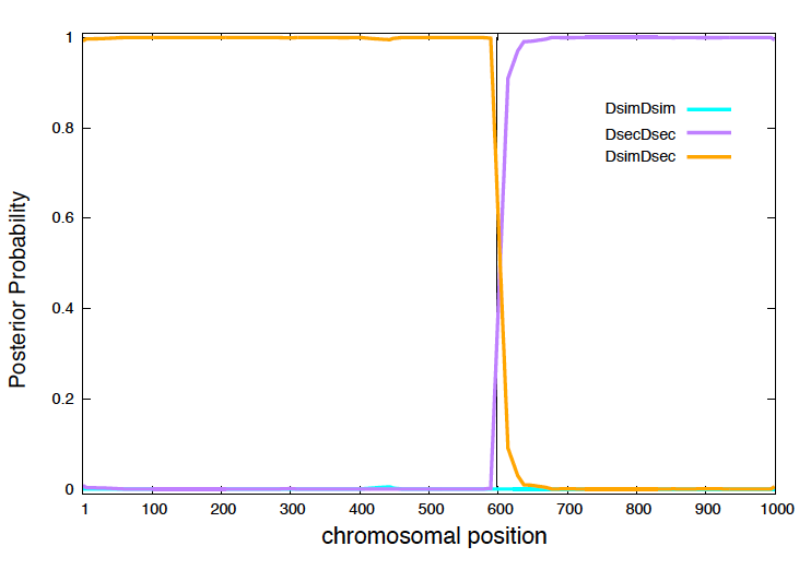
Figure 4. Posterior probabilities for a male fly backcross in a 1,000 nucleotides region.
I have simulated mapped reads for a male fly backcross
\[\mbox{Dsim/Dsec} \times \mbox{Dsec/Dsec},\]and a hypothetical region of 1,000 bases, where I introduced one breakpoint.
In Figure 4, I display for each position \(1\leq i\leq 1000\), the three posterior probabilities
\[P(Z_i=\mbox{Dsim}/\mbox{Dsim}),\\ P(Z_i=\mbox{Dsec}/\mbox{Dsec}),\\ P(Z_i=\mbox{Dsec}/\mbox{Dsim}),\\\]obtained using the posterior decoding algorithm.
The posterior probabilities, clearly indicate the presence of two regions Dsim/Dsec and Dsec/Dsec, with one breakpoint (and only one) occurring around position 600. As expected, due to the nature of the backcross the posterior probability of having ancestry Dsim/Dsim are zero at every position.