MCB111: Mathematics in Biology (Fall 2024)
- Chemical reactions
- Transcriptional activation
- Transcriptional inhibition
- Transcription summary
- Simplest Feedback loop: Autoregulation
- Gene regulation with a negative feedback loop
- Gene regulation with a positive feedback loop
week 11:
Feedback Control in Biological Interactions
For these lectures, I have followed many different sources. Some of them are: Chapter 9 of P. Nelson’s book, “Biochemical oscillations” by J. Tyson, the paper “Chemical and enzymatic kinetics” by D. Gonze, “Positive feedback in cellular control systems” by Mitrophanov & Grossman.
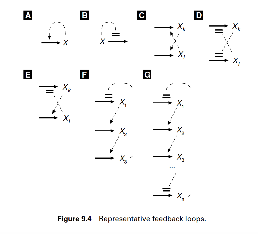
Figure 1. Solid arrows represent chemical reactions producing or consuming compounds. Dashed arrows represent regulatory signals: a modification to the chemical reaction by a species which concentration's that may not be substrate or product of the reaction. Regulatory signals end with either an arrow (indicating activation) or with a blunt end (indicating inhibition). Figure from J. Tyson's "Biochemical oscillations"
Feedback loops occur in many different biological systems. From gene regulation, RNA and protein production, protein phosphorylation, catalysis, to cell cycle and circadian rhythms. Feedback loops can be positive or negatives, and they give raise to many different behaviors: stable, unstable, cyclic, oscillatory, hysteresis, etc.
Here are some examples of feedback loops from J. Tyson’s paper.
Chemical reactions
This is some background on chemical reactions which are the building blocks of any feedback loop.
Consider four different compounds A, B, C, D (these could be enzymes, RNA, transcription factors,…). Assume that they such that the interaction of A and B produce the compounds C and D,
\[A+ B\overset{k}{\longrightarrow} C+D\]where A, B, C, and D, in the above equation represent the concentration (that is, the average number of molecules per unit volume) of the different compounds.
In a chemical reaction, there is stochasticity as the molecules have to collide to interact, but not all collisions are successful. The probability that one collision is successful is given by \(k\) which represent the probability of change per time unit. The number of collisions is proportional to the concentration of the substrates A and B, so the rate of the reaction is going to be proportional to the quantity
\[v = k A B\]which is referred to as the mass action law.
The change with time of the concentrations of the different compounds is given by
\[\begin{aligned} \frac{d A}{d t} = \frac{d B}{d t} &= -k\ A B\\ \frac{d C}{d t} = \frac{d D}{d t} &= +k\ A B. \end{aligned}\]The sign in the right hand side of the equations indicate that every time the reaction proceeds, one molecule of substrates A and B disappears and one molecule of products C and D appears. These results can be derived from the master equations similarly to how we derived those of the average concentration of RNA in the previous week. You can find the derivation in the sections.
The variation in the concentrations of the four species governed by these differential equations for some particular starting concentrations is given in Figure 2.
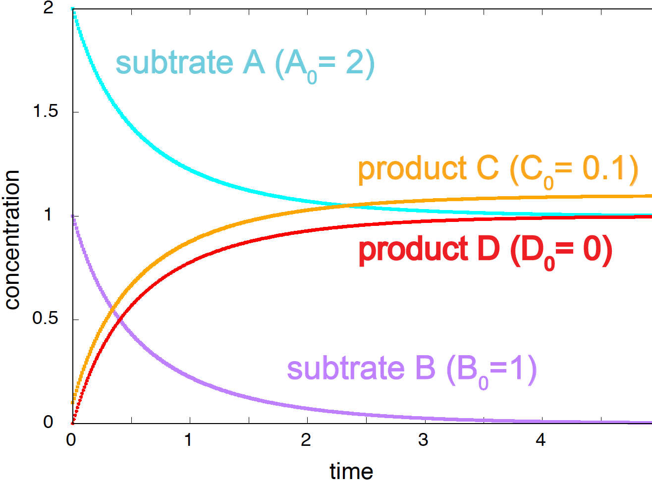
Figure 2. Time evolution of the concentrations of species A, B, C, and D, for the rate constant value k=1.0.
Evolution equation for a general reaction
In general, for one reaction with \(N\) substrates \(X_1,\ldots X_N\),
\[n_1 X_1 + \ldots + n_N X_N \overset{k}{\longrightarrow} p_1 X_1 + \ldots + p_N X_N\]the mass action law is given by
\[v = k\ (X_1)^{n_1}\ldots (X_N)^{n_N} = k\ \prod_{i=1}^N (X_i)^{n_i}\]and the change with time of one species \(X_i\) is given by
\[\frac{d X_i}{d t} = (p_i-n_i)\ v = \eta_i\ v.\]were \(\eta_i = p_i -n_i\) is the stoichiometric coefficient.
Examples
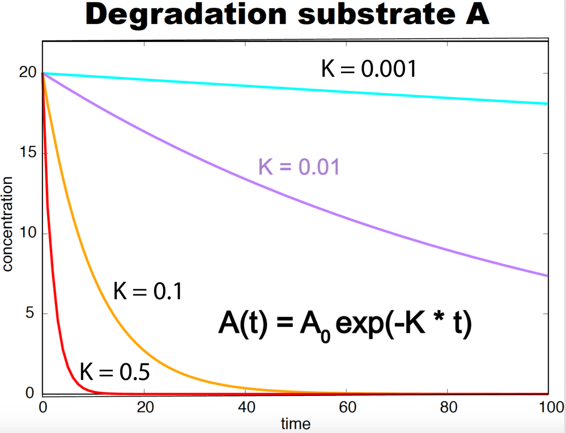
Figure 3. Degradation curves as a function of time for a substrate A with different rate constants (k). The concentration of A at time zero is 20.
-
Degradation, conformational change, or dissociation
\[\begin{aligned} A\overset{k}{\longrightarrow} \emptyset&\quad\mbox{Degradation}\\ or\\ A\overset{k}{\longrightarrow} A^\ast&\quad\mbox{Conformational change}\\ or\\ A\overset{k}{\longrightarrow} B + C&\quad\mbox{Dissociation} \end{aligned}\]follow the same dynamics for the substrate \(A\)
\[\frac{d A}{d t} = - k A.\]After integrating
\[A(t) = A_0 e^{-k t},\]where \(A_0\) is the concentration of species \(A\) at time zero, see Figure 2.
-
Cooperative
\[3 A \overset{k}{\longrightarrow} C + A\]Three molecules of species \(A\) are required to produce species \(C\), but one of molecule of species \(A\) is conserved, resulting in the equation
\[\frac{d A}{d t} = -2 k A^3\]
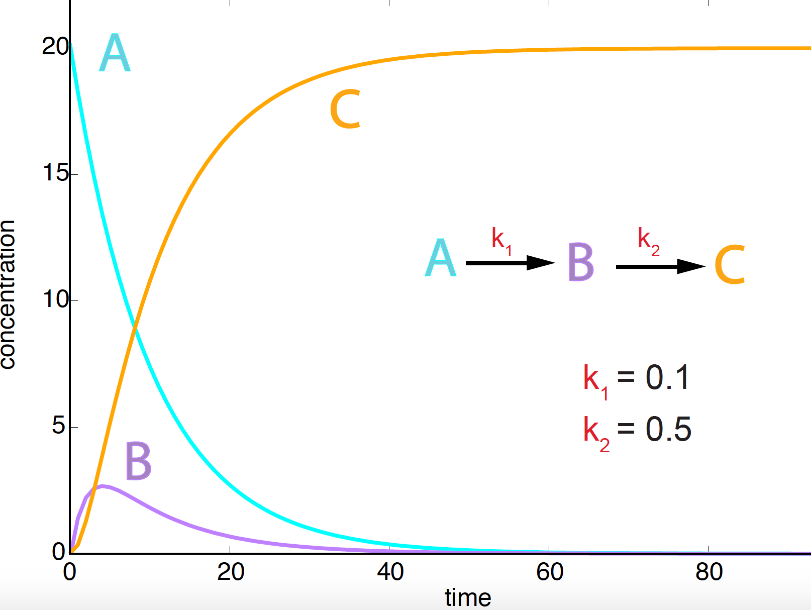
Figure 4. Concentration evolution curves as a function of time for two serial reactions involving three species A, B, C. Starting concentrations are 20, 0, 0 respectively.
-
Serial reactions
\[A \overset{k_1}{\longrightarrow} B \overset{k_2}{\longrightarrow} C\]The dynamics is given by
\[\begin{aligned} \frac{d A}{d t} &= -k_1\ A\\ \frac{d B}{d t} &= k_1\ A - k_2\ B\\ \frac{d C}{d t} &= k_2\ B. \end{aligned}\]We can obtain an analytic solution for this process, see Figure 4, given by
\[\begin{aligned} A(t) &= A_0\ e^{-k_1\ t}\\ B(t) &= \frac{A_0\ k_1}{k_2 - k_1}\ \left( e^{-k_1\ t} - e^{-k_2\ t}\right)\\ C(t) &= A_0\ \left[1-\frac{1}{k_2-k_1}\left( k_2\ e^{-k_1\ t} - k_1\ e^{-k_2\ t} \right)\right], \end{aligned}\]under the initial conditions \(A(t=0) = A_0, B(t=0) = 0\), and \(C(t=0)=0\).
The degradation of species \(A\) has not changed. Species \(B\) increases its concentration for a while until it starts being used to produce species \(C\). After a very long time, the concentration of species \(A\) and \(B\) is zero, and \(C\) reaches the starting concentration of species \(A\) (\(A_0 = 20\)).
Multiple reactions
And for \(R\) reactions involving \(N\) substrates \(X_1\ldots X_N\), with rate constants \(k_1,\ldots k_R\),
\[\begin{aligned} n^1_1\ X_1 + \ldots + n^1_N\ X_N &\overset{k_1}{\longrightarrow} p^1_1 X_1 + \ldots + p^1_N X_N\\ \vdots\\ n^R_1\ X_1 + \ldots + n^R_N\ X_N &\overset{k_R}{\longrightarrow} p^R_1 X_1 + \ldots + p^R_N X_N \end{aligned}\]the contribution of the different reactions is additive,
\[\begin{aligned} \frac{d X_i}{d t} &= (p^1_i-n^1_i)\ k_1 (X_1)^{n^1_1}\ldots (X_N)^{n^1_N} + \ldots + (p^R_i-n^R_i)\ k_R (X_1)^{n^R_1}\ldots (X_N)^{n^R_N}\\ &= \sum_{r=1}^R (p^r_i-n^r_i)\ k_r (X_1)^{n^r_1}\ldots (X_N)^{n^r_N}\\ &= \sum_{r=1}^R (p^r_i-n^r_i)\ k_r \prod_{j=1}^{N}(X_j)^{n^r_j}\\ &= \sum_{r=1}^R \eta^r_i\ v_r. \end{aligned}\]where \(\eta^r_i\) is the stoichiometry of species \(X_i\) in reaction \(r\), and \(v_r\) is the mass action law of reaction \(r\).
Transcriptional activation
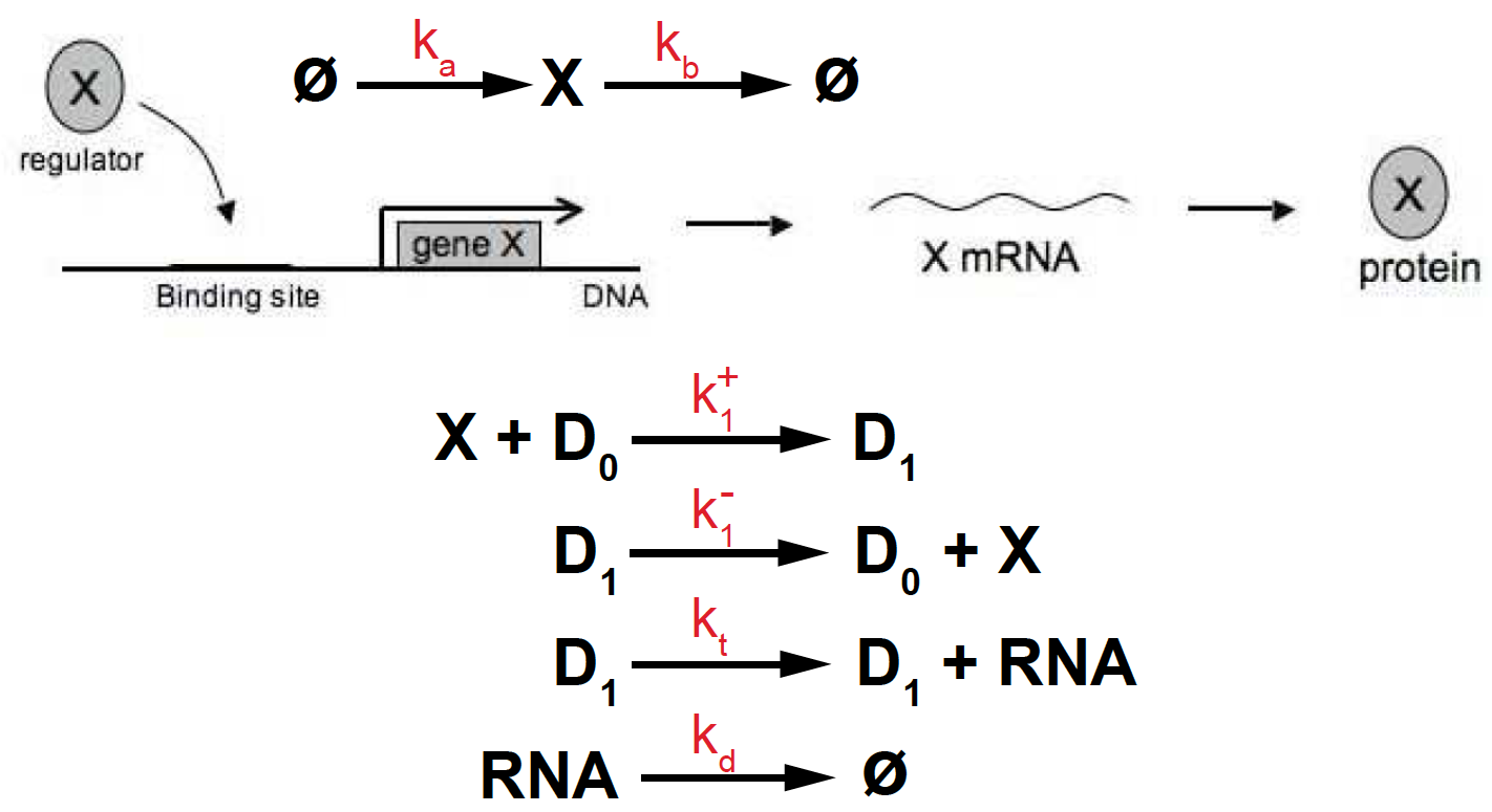
Figure 5. Transcriptional activation depending on one binding site.
One binding site
Let’s assume that the activation of a gene that produces a RNA, requires one particular transcription factor (X) to bind to one specific binding site upstream of the gene.
Let’s assume the following
-
We describe as \(D_1\) the state of the gene such that X is bound and transcription occurs. Let’s \(k^+_1\) be the rate of X binding.
-
We describe as \(D_0\) the gene state such that X is not bound and transcription does not occur. The TF binding to the gene is reversible. Let’s \(k^-_1\) be the rate of X unbinding, leaving the gene inactive in state \(D_0\).
-
Production of the RNA is only possible when the transcription factor is bound (state \(D_1\)). When the gene is in \(D_1\) state, RNA transcription occurs with rate \(k_t\).
-
The transcription factor (X) has some known rates of production (\(k_a\)) and degradation (\(k_b\)).
-
The RNA is also subject to degradation with rate \(k_d\).
-
The rates of TF binding/unbinding \(D_1 \leftrightarrow D_0\) are fast (several times per second), while the rate of transcription is much slower (it can take up to several minutes). Thus,
The reactions describing this process of transcriptional activation with one binding site are:
\[\begin{aligned} \emptyset\overset{k_a}{\longrightarrow} X &\quad\mbox{TF production}\\ X \overset{k_b}{\longrightarrow} \emptyset &\quad\mbox{TF degradation}\\ X + D_0 \overset{k^+_1}{\longrightarrow} D_1 &\quad\mbox{TF binding}\\ D_1 \overset{k^-_1}{\longrightarrow} D_0 + X &\quad\mbox{TF unbinding}\\ D_1 \overset{k_t} {\longrightarrow} D_1 + RNA &\quad\mbox{RNA production (transcription)}\\ RNA \overset{k_d} {\longrightarrow} \emptyset &\quad\mbox{RNA degradation}. \end{aligned}\]Figure 6. (A) Transcription rate (dRNA/dt) for one activation binding site. (B) Transcription rate (dRNA/dt) in the presence of two activation binding sites both cooperative (purple) and non-cooperative (yellow). (C) Transcription rate (dRNA/dt) in the presence of an arbitrary number of activation binding sites. Parameter values are v=1 and K=1.5.
The corresponding kinetic equations (following the general rule described above) are
\[\begin{aligned} \frac{d X}{d t} &= k_a - k_b X - k^+_1 X D_0 + k^-_1 D_1\\ \frac{d D_1}{d t} = -\frac{d D_0}{d t} &=k^+_1 X D_0 - k^-_1 D_1\\ \frac{d RNA}{d t} &= k_t D_1 - k_d RNA. \end{aligned}\]The assumption that the binding/unbinding of the TF is very fast compared to that of the production of RNA, implies that by the time binding/unbinding has reached equilibrium, the transcription kinetics is still underway. Thus, we can make the assumption that binding/unbinding has reached steady state
\[\frac{d D_1}{d t} = -\frac{d D_0}{d t} = 0\]That is
\[k^+_1 X D_0 = k^-_1 D_1.\]Introducing \(D_T = D_0+D_1\) as the
\[k^+_1 X (D_T-D_1) = k^-_1 D_1.\]or
\[D_1 = \frac{k^+_1 X D_T}{k^-_1+k^+_1 X}.\]Let’s introduce the dissociation equilibrium constant
\[K_1 = \frac{k^-_1}{k^+_1}\] \[D_1 = D_T\ \frac{X}{K_1+X}.\]Under this assumption of binding/unbinding steady state, the remaining equations become
\[\begin{aligned} \frac{d X}{d t} &= k_a - k_b X\\ \frac{d RNA}{d t} &= k_t D_T\ \frac{X}{K_1+X} - k_d RNA. \end{aligned}\]That is,
-
The kinetics of the TF depends only on its own synthesis and degradation
\[\frac{d X}{d t} = k_a - k_b X\] -
The concentration of RNA for fast binding/unbinding of one activator (X) is then given by
\[\frac{d RNA}{d t} = k_t D_T\ \frac{X}{K_1+X} - k_d RNA.\]That is, the transcription process is controlled by the activator concentration (X) according to the equation
\[\frac{d RNA}{d t} = v\ \frac{X}{K_1+X}\]where \(v=k_t D_T\) is a constant. This is a hyperbolic curve referred to as a non-cooperative binding curve (see Figure 6A).
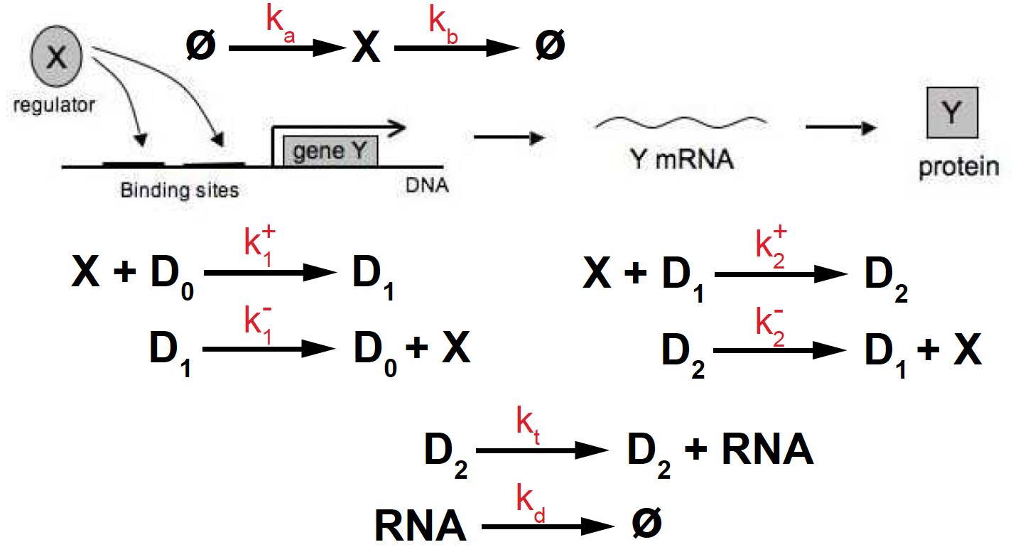
Figure 7. Transcriptional activation depending on two binding sites.
Multiple binding sites
Now let’s assume that the gene has two binding sites upstream of the transcription start site. The activator (X) has to bind to both sites for transcription to occur, then the reactions controlling transcription are given by (see Figure 7)
\[\begin{aligned} \emptyset\overset{k_a}{\longrightarrow} X \overset{k_b}{\longrightarrow} \emptyset &\quad\mbox{TF production/degradation}\\ X + D_0 \underset{k^-_1}{\overset{k^+_1}{\rightleftharpoons}} D_1 &\quad\mbox{TF binding/unbinding to one site}\\ X + D_1 \underset{k^-_2}{\overset{k^+_2}{\rightleftharpoons}} D_2 &\quad\mbox{TF binding/unbinding to second site}\\ D_2 \overset{k_t} {\longrightarrow} D_2 + RNA &\quad\mbox{RNA production (transcription)}\\ RNA \overset{k_d} {\longrightarrow} \emptyset &\quad\mbox{RNA degradation}. \end{aligned}\]And the kinetic equations are given by
\[\begin{aligned} \frac{d X}{d t} &= k_a - k_b X - k^+_1 X D_0 + k^-_1 D_1 - k^+_2 X D_1 + k^-_2 D_2\\ \frac{d D_0}{d t} &= k^-_1 D_1 - k^+_1 X D_0\\ \frac{d D_1}{d t} &= k^+_1 X D_0 - k^-_1 D_1 - k_2^+ X D_1 + k_2^- D_2\\ \frac{d D_2}{d t} &= k_2^+ X D_1 - k_2^- D_2\\ \frac{d RNA}{d t} &= k_t D_2 - k_d RNA. \end{aligned}\]If we assume that the binding/unbinding kinetics is much faster than transcription, we can assume steady state
\[\frac{d D_0}{d t} = \frac{d D_1}{d t} = \frac{d D_2}{d t} = 0\]which implies that
\[k^-_1 D_1 = k^+_1 X D_0\\ k^-_2 D_2 = k^+_2 X D_1.\]Introducing the disequilibrium constants \(K_1 = k^-_1/k^+_1\) and \(K_2 = k^-_2/k^+_2\), we obtain
\[\begin{aligned} D_1 &= \frac{X D_0}{K_1}\\ D_2 &= \frac{X D_1}{K_2} = \frac{X^2 D_0}{K_1 K_2}. \end{aligned}\]Introducing \(D_T = D_0 + 2 D_1 + D_2\) which is the total number of genes per unit volume (since when binding to one site, it could be either of the two sites), we have
\[D_T = D_0 + 2\frac{X D_0}{K_1} + \frac{X^2 D_0}{K_1 K_2} = D_0\left(1+2\frac{X}{K_1} + \frac{X^2}{K_1 K_2}\right)\]or
\[D_0 = \frac{D_T}{1+2\frac{X}{K_1} + \frac{X^2}{K_1 K_2}}.\]Then the kinetics of transcription is given by
\[\frac{d RNA}{dt} = k_t D_2 = k_t \frac{X^2 D_0}{K_1 K_2} = k_t \frac{D_T \frac{X^2}{K_1K_2}}{1+2\frac{X}{K_1} + \frac{X^2}{K_1 K_2}}\]We can now distinguish two situation:
Non-cooperative binding
Under non-cooperative binding, the two sites load independently with the same rates, thus, \(K_1 = K_2 = K\). Then the kinetics of transcription is given by
\[\begin{aligned} \frac{d RNA}{dt} &= k_t \frac{D_T X^2/K^2}{1+2 X/K + X^2/K^2}\\ &= k_t D_T \left(\frac{X/K}{1+X/K}\right)^2 \end{aligned}\]In Figure 6B, we compare the dynamics of two independent (non-cooperative) binding sites (in yellow) to that of one binding site (cyan).
Cooperative binding: The Hill Function
If the binding to the two sites is cooperative, that means, that the binding of the second site is faster than that of the first one, that is \(k_2^+ >> k_1^+\), and \(k_2^- \sim k_1^-\). That translate into \(K_2 = \frac{k_2^-}{k_2^+} << K_1 = \frac{k_1^-}{k_1^+}\).
Under cooperative binding conditions, we can introduce a parameter \(K\) defined by
\[K_2 = \frac{K^2}{K_1}\]such that \(K\) is finite, and \(K_2 \rightarrow 0\) as \(K_1 \rightarrow \infty\).
Then
\[\frac{d RNA}{dt} = k_t D_T\frac{\left(\frac{X}{K}\right)^2}{1+2\frac{X}{K_1} + \left(\frac{X}{K}\right)^2}\]since cooperative binding implies that \(K_1 >> K\), we can approximate the above expression as
\[\frac{d RNA}{dt} \approx k_t D_T \frac{\left(\frac{X}{K}\right)^2}{1+\left(\frac{X}{K}\right)^2}\]which can be re-written as
\[\frac{d RNA}{dt} \approx v \frac{X^2}{K^2+X^2}\]where \(v = k_t D_T\) is a constant. This function is referred to as a Hill equation with Hill coefficient \(n=2\).
In Figure 6B, we compare the dynamics of two cooperative binding sites (in purple) to that of two independent (non-cooperative) binding sites (in yellow), and one binding site (cyan).
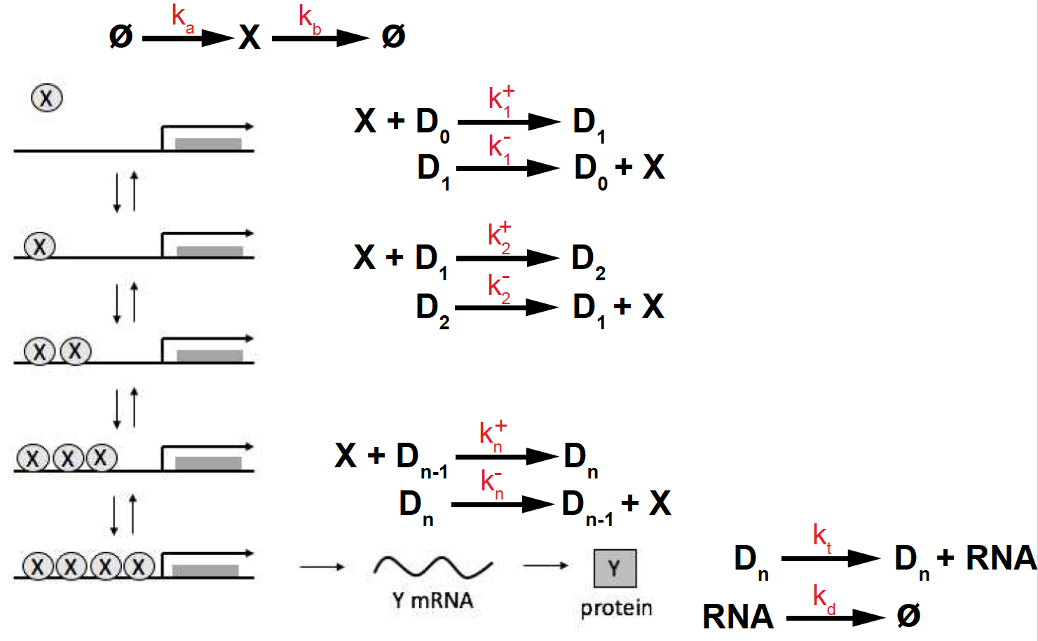
Figure 8. Transcriptional activation depending on multiple binding sites.
In the case of many (\(n\)) cooperative biding sites (see Figure 8), the above expression generalizes to
\[\frac{d RNA}{dt} = v \frac{X^n}{K^n+X^n}\]In Figure 6C, we show different Hill functions for different cases of cooperative binding sites. We observe that under cooperative binding, less amount of the activator is required for the rate of transcription to reach is maximum value.
Transcriptional inhibition
Transcription can also be inhibited by binding of an inhibitor. If X acts as a transcriptional inhibitor, we have the following reaction scheme,
\[\begin{aligned} \emptyset\overset{k_a}{\longrightarrow} X \overset{k_b}{\longrightarrow} \emptyset &\quad\mbox{X production/degradation}\\ X + D_0 \underset{k^-_1}{\overset{k^+_1}{\rightleftharpoons}} D_1 &\quad\mbox{X binding/unbinding}\\ D_0 \overset{k_t} {\longrightarrow} D_0 + RNA &\quad\mbox{Transcription only in the absence of X} \end{aligned}\]where transcription only occurs in the absence of the inhibitor X.
And the kinetic equations are given by
\[\begin{aligned} \frac{d X}{d t} &= k_a - k_b X - k^+_1 X D_0 + k^-_1 D_1\\ \frac{d D_0}{d t} = - \frac{d D_1}{d t} &= k^-_1 D_1 - k^+_1 X D_0\\ \frac{d RNA}{d t} &= k_t D_0. \end{aligned}\]Under steady state \(\frac{d D_0}{d t} = \frac{d D_1}{d t} = 0\), we have
\[D_0 = K_1 \frac{D_1}{X}\]where \(K_1 = k^-_1/k^+_1\). Introducing \(D_T = D_0 + D_1\), we obtain
\[\frac{dRNA}{d t} = k_t D_T \frac{K_1/X}{1+ K_1/X} = v \frac{K_1}{K_1+X}\]for \(v = k_t D_T\).
This generalizes for multiple inhibitory sites as
\[\frac{dRNA}{d t} = v \frac{K_1^n}{K_1^n+X^n}\]which is also a Hill equation.
In Figure 9, we show the effect in transcription rate of inhibition under different degrees of cooperativity. Reciprocally to activation, as cooperativeness increases, less inhibitor is required to achieve the same rate of inhibition.
Figure 9. Transcription inhibition. parameters are v=1 and K=1.5.
Transcription summary
Here is a summary of the simplified kinetics of transcription regulation that we have discussed so far.
| Type | Trascription rate dRNA/dt | |
| Activation 1 site | \(v\frac{X}{K+X}\) | Figure 6A |
| Activation n sites/uncooperative | \(v\left(\frac{X}{K+X}\right)^n\) | Figure 6B |
| Activation n sites/cooperative | \(v\frac{X^n}{K^n+X^n}\) | Figure 6C |
| Inhibition n sites/cooperative | \(v\frac{K^n}{K^n+X^n}\) | Figure 9 |
where \(X\) is the TF concentration, and \(K\) the dissociation equilibrium constant which describes the strength of the binding.
Simplest Feedback loop: Autoregulation
In autoregulation, a protein (a transcription factor) represses (or activates) the transcription of its own gene. This is an important mechanism, for instance negative autoregulation occurs in 40% of E. coli transcription factors (Rosenfeld et. al).
Autoregulation can be simple (no feedback loop) or involving a feedback look by which the species either activates (positive feedback) or inhibits (negative feedback) its own production. Figure
- gives a graphical representation of these simple feedback loops.
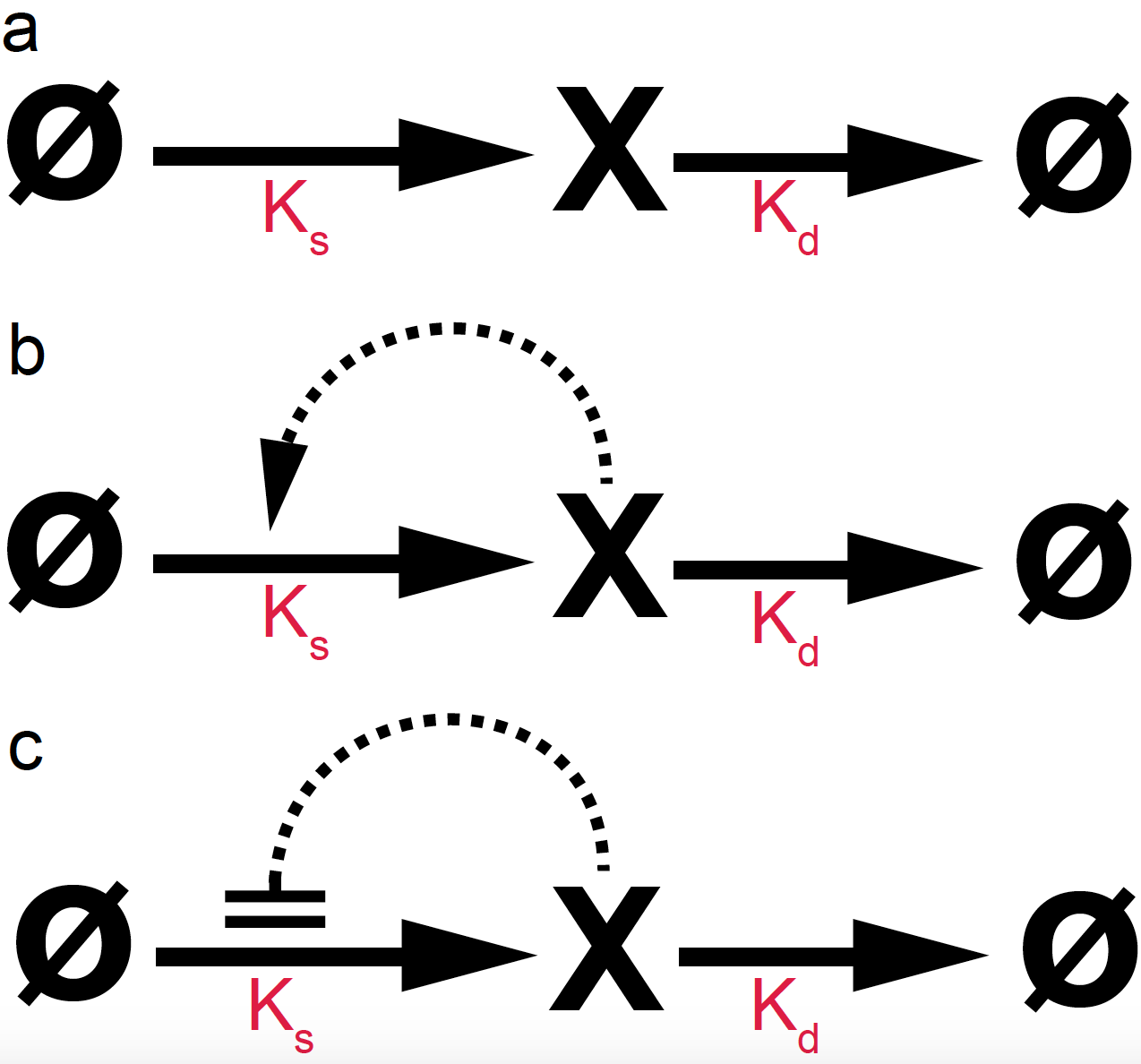
Figure 10. Autoregulation with simple (a), a positive feedback loop (b) and a negative loop (c).
The kinetic equations for the autoregulation of a species X is given by
| Type | Concentration change with time |
| simple regulation | \(dX/dt = k_s - k_d X\) |
| negative autoregulation | \(dX/dt = k_s \frac{K^n}{K^n+X^n} - k_d X\) |
| positive autoregulation | \(dX/dt = k_s \frac{X^n}{K^n+X^n} - k_d X\) |
where we have used Hill functions to describe the positive and negative feedback loops.
The differential equation for the simple regulation case has an analytical solution given by
\[X(t) = \frac{k_s}{k_d} \left(1-e^{-k_d t}\right)\quad \mbox{simple autoregulation}.\]However most differential equations do not have analytical solutions, but good approximate solutions can be found numerically.
Numerical Solutions for ordinary differential equations (ODEs): The Euler Method
The autoregulation differential equations belong to the category of ordinary differential equations (ODE).
Many different numerical methods exist to solve ODEs. Numerical methods to solve differential equations were introduced a long time before computers. Next I will discuss one of the simplest methods, the Euler method, which dates to Leonhard Euler (1707-1783).
You can find different packages to solve ODES, such as XPP, and several matlab packages to name a few. A good review of methods and software packages that implement them is this report “Numerical methods for ordinary differential equations’.
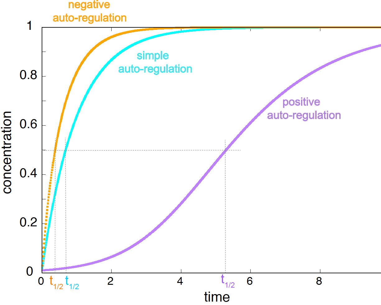
Figure 11. Simple autoregulation (cyan), negative autoregulation (yellow), and positive autoregulation (purple). Parameters are K = 1; ks=1 for the simple method and ks=2 for both positive and negative autoregulation, and kd=1 for all three cases. The Hill coefficient for both feedback loops is n=1. Original concentration at t=0 is 0.01 for all three methods.
Even if you decide to use a package for your work, I would recommend that you implement your own at least once so you understand the details, and are better prepared to assign parameter values when you decide to move to use a given package. The Euler method what we as showing next is the simplest, and it just simply discretizes the meaning of a derivative.
Consider a differential equation for variable \(X\)
\[\frac{d X}{d t} = f(t,X).\]By a numerical solution we understand, starting from a known value \(X_0\) at \(t_0\), to calculate \(X_1\), \(X_2\), \(X_3\), at times \(t_1=t_0+\Delta t\), \(t_2=t_0+2\Delta t\ldots\)
The Euler method, updates those values as
\[X_{n+1} = X_{n} + \Delta t * f(t_n,X_n)\]The value of \(\Delta t\) is arbitrary. The smaller you make \(\Delta t\) the better your recursion will approximate the actual continuous derivative. In Figure 11, I have used \(\Delta t = 0.01\).
Autoregulation controls the response time of the system
Applying the Euler method to the positive and negative autoregulation feedback networks results in Figure 11.
-
Negative autoregulation speeds up the response time relative to the simple case, and steady state is reached faster. Many biological examples have been studied of negative autoregulation, particularly in bacteria. Here is an example, “Negative autoregulation speeds the response times of transcription networks.” by Rosenthal et al..
-
Positive autoregulation slows down the response time relative to the simple case, and the steady state is reached at a later time. Positive autoregulation has been designed in experimental systems, for which the mathematical models fit well the observed data. Here is an example, “Regulatory dynamics of synthetic gene networks with positive feedback” by Maeda & Sano.
Gene regulation with a negative feedback loop
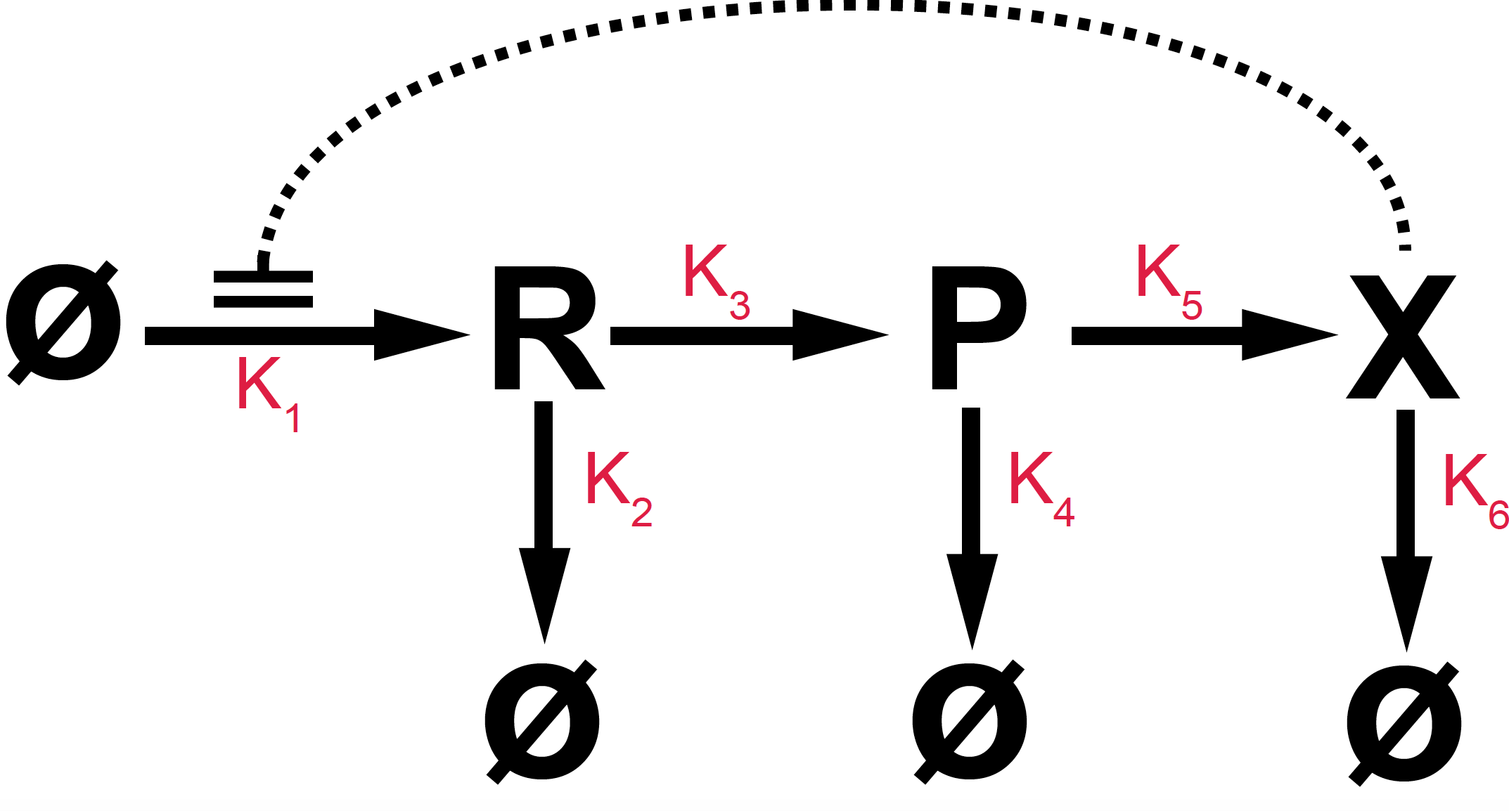
Figure 12. The Goodwin model is a negative feedback loop. Species X modifies transcription (R) by a negative feedback loop that we model by a non-linear Hill function.
The Goodwin model was introduced by B. Goodwin in 1965 in this work “Oscillatory behavior in enzymatic control process”. The Goodwin model is the prototype of a negative feedback loop that produces interesting behaviors (in this case oscillations).
In the Goodwin model a gene produces a species of RNA (R) which in turn produces a protein (P). The protein (P) is involved in some metabolic process which results in the production of another protein (X), which acts as an inhibitor in the production of the RNA.
The reactions for the Goodwin model are given in Figure 12. The associated differential equations are
\[\begin{aligned} \frac{d R}{dt} &= k_1 \frac{K^n}{K^n+X^n} - k_2 R\\ \frac{d P}{dt} &= k_3 R - k_4 P\\ \frac{d X}{dt} &= k_5 P - k_6 X \end{aligned}\]where we have modeled the negative feedback loop that the protein X exerts on transcription by a Hill function.
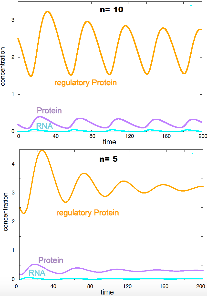
Figure 13. Dynamics of the Goodwin model. Parameters are k1=k3=k5=1, k2=k4=k6=0.1, K = 1. Initial concentrations are R = 0, P=0.2, X = 2.5.
Negative feedback loops produce oscillations
The behavior of the Goodwin model can be seen in Figure 13, where I have solved numerically the differential equations for some particular values of the parameters. The Goodwin model shows periodic oscillations for \(n>8\). For \(n<8\) the oscillations are dampened.
This is the first model that showed oscillations at the molecular level. Oscillation in molecular biology systems are well documented, and it is important to have mathematical models that reproduce them.
The Hill coefficient \(n\) represents the degree of cooperativeness, that is how many molecules of regulator \(X\) bind to the promoter region. The Goodwin model has been criticized because a cooperativity of \(n>8\) is very high and unrealistic for most biological situations. There is more recent work trying to lower the non-linearity requirement in order to obtain oscillatory behaviors, for instance by adding phosphorylation/de-phosphorylation processes, as in with work by Gonze & Abou-Jaoude.
Gene regulation with a positive feedback loop
Positive feedback loops have some other interesting properties relative to negative loops such as, bistability, hysteresis, and activation surges. Here I follow the work of Mitrophanov & Groisman “Positive feedback in cellular control systems”.
The PhoP/PhoQ system
In the PhoP/PhoQ operon in bacterium Salmonella enterica, there is a positive feedback loop. The operon has a constitutive promoter, and another promoter that can be induced by the presence of PhoP in phosphorylated form (Figure 14).
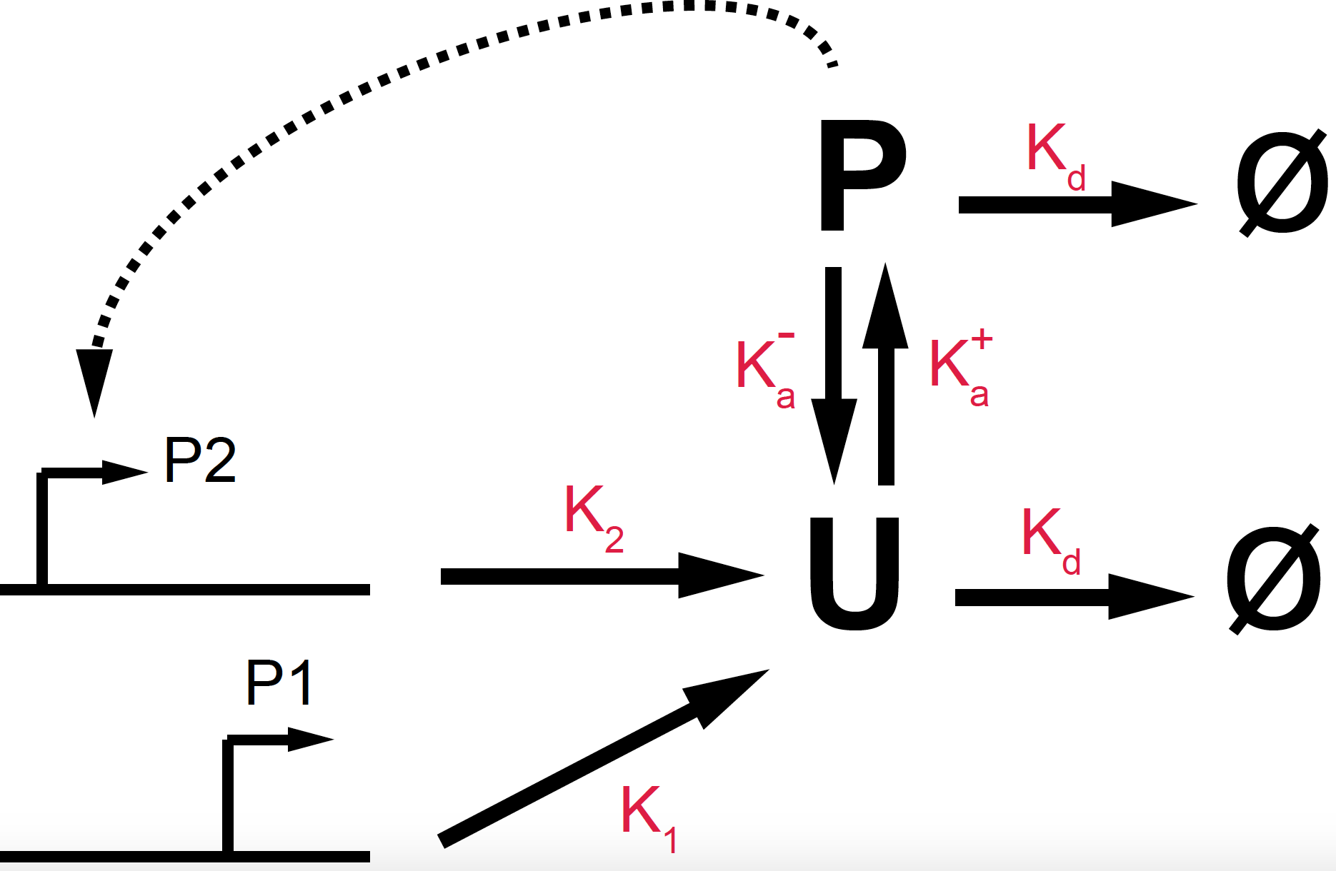
Figure 14. Diagrammatic representation of the PhoP phosphorylation/de-phosphorylation positive feedback loop.
The differential equations are given by
\[\begin{aligned} \frac{d U}{dt} &= k_1 + k_2 \frac{P^n}{K^n+P^n} + k^-_a P - (k_d + k^+_a) U\\ \frac{d P}{dt} &= k^+_a U - (k_d + k^-_a) P \end{aligned}\]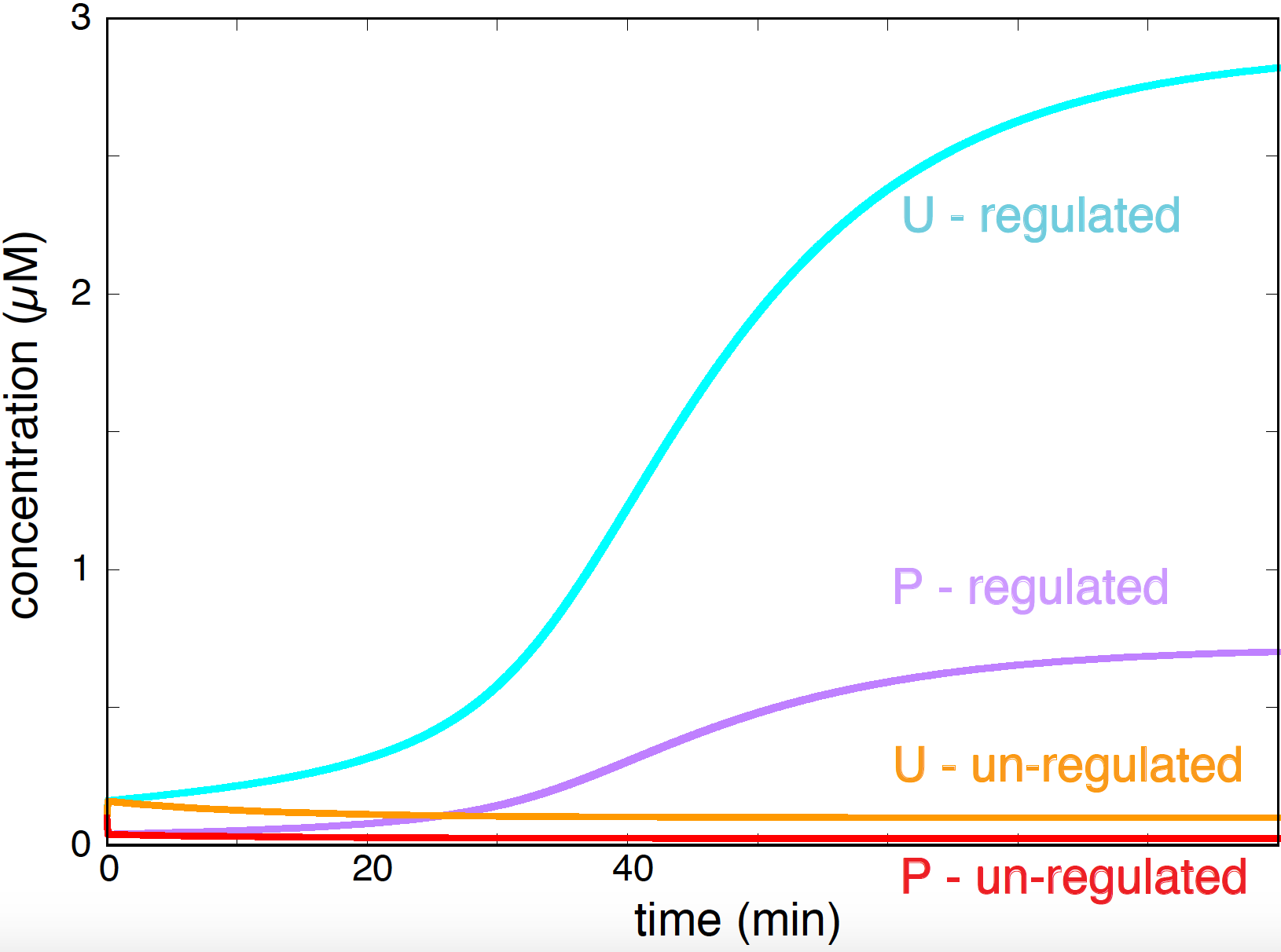
Figure 15. Effect in protein concentration due to the presence of a inducible promoter. Parameters are: k1=0.01, k2 = 0.3, ka+ = 5 ka- = 20, kd = 0.08, K=0.2, n=2, for time measured in minutes and concentrations in microM.
where P stands for the phosphorylated form of PhoP, and U stands for the un-phosphorylated form of PhoP. \(k_1\) is the rate of the constitutive promoter, and \(k_2\) the rate of the inducible promoter. We have modeled the positive feedback induced by the phosphorylated form of PhoP by a Hill function. \(k^+_a\) and \(k^-_a\) are the rates of exchange between the phosphorylated and un-phosphorylated forms. Both forms of the protein degrade with rate \(k_d\).
In the absence of the inducible promoter (\(k2=0\)), and using parameters close to the biological conditions, both concentration of the phosphorylated and unphosphorylated form of the protein are very low. By contrast, when the inducible promoter is turned on, the phosphorylated protein activates the inducible promoter and the concentrations of both states of protein PhoP increase drastically (Figure 15).
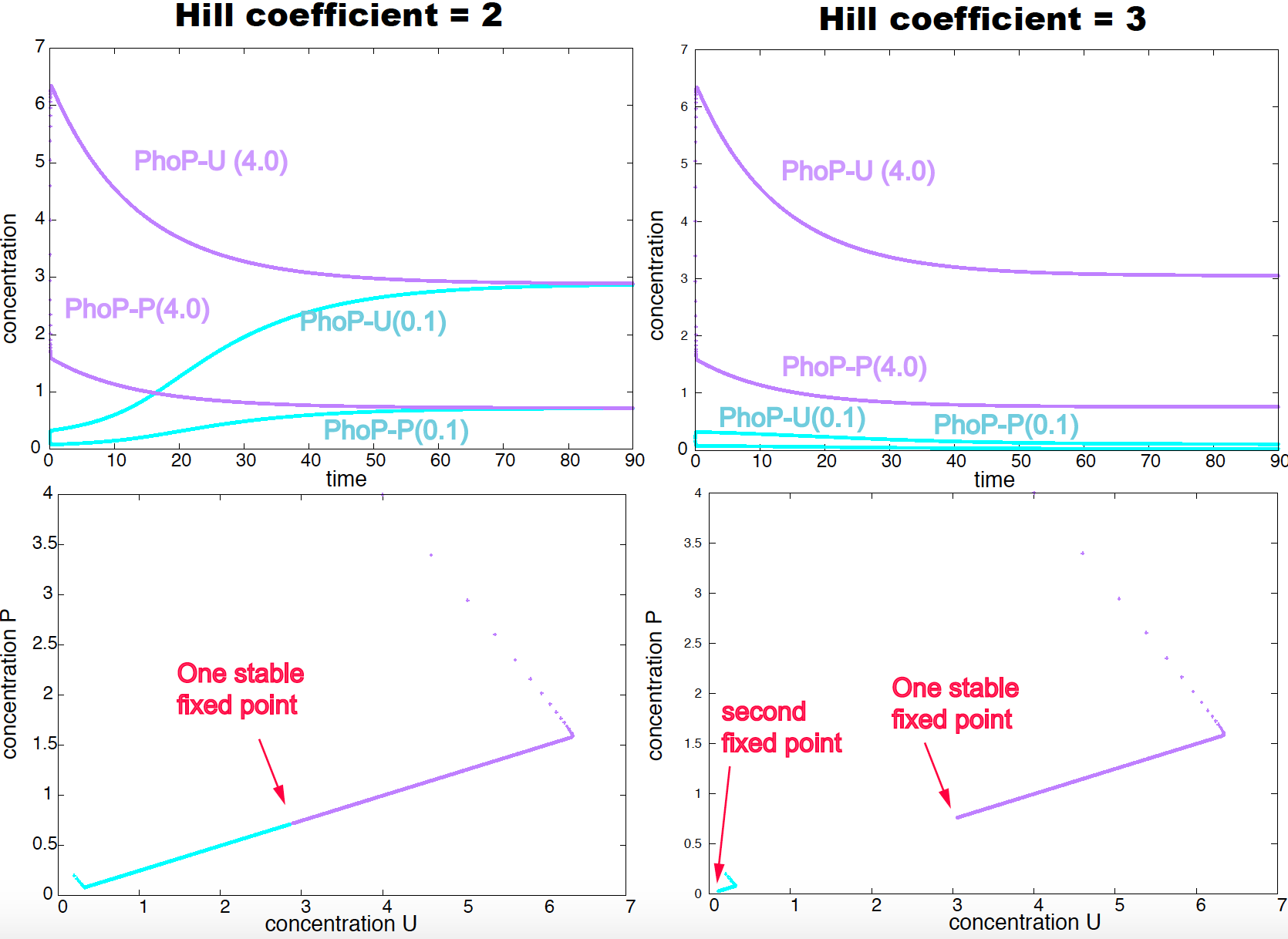
Figure 16. The positive feedback loop of PhoP (with the same biologically relevant parameters than in Figure 15), shows only one steady state under a Hill coefficient of 2 (left-hand side panels), but two different steady states (bistability) when the Hill coefficient is 3 (right-hand side panels). In purple trajectories starting from an initial concentration of 4.0 (for both forms of the protein). In blue trajectories starting from an initial concentration of 0.1 (for both forms of the protein).
Positive Feedback produces bistability
A system is called bistable if it can reach different steady states depending of the initial conditions of the system. Positive feedback loops can provide bistable solutions. The PhoP/PhoQ system, under biological relevant parameters, exhibits bistatiblity for cooperative factor \(n=3\), but not for \(n=2\).
In Figure 16, we show for the same parameter conditions than in Figure 15, we compare the evolution of the concentrations of the phosphorylated and un-phosphorylated forms of the protein PhoP starting from two different concentrations: 4.0, 4.0 (in purple) and 0.1, 0.1 (in blue). While both initial conditions.
The second steady state corresponds to very small concentrations of the protein. This is a known phenomena. For instance, the E. coli lactose utilization system (the Lac Operon) has two different steady states, one achieving high concentrations, and the other very small concentrations.