MCB111: Mathematics in Biology (Fall 2024)
week 05:
Maximum likelihood and least squares
For this topic, I will follow Sivia’s Chapters 3 and 5. One of the first instances of using Maximum likelihood for quantitative trait loci mapping is this Lander and Botstein paper from 1988 “Mapping mendelian factors underlying quatitative traits loci using RPLF linkage maps.”
Maximum Likelihood
We have used Bayes theorem to calculate the probability of the parameters (\(X\)) of a given hypothesis (\(H\)) given the data (\(D\)) as
\[P(X\mid D, H) \propto P(D\mid X, H)\, P(X\mid H)\]where \(P(X\mid H)\) is the prior probability of the parameters.
We have seen some examples in which we have calculated the posterior probability distribution explicitly. Oftentimes we get away with just finding the parameter values that maximize the posterior probability.
If we do not have any information before doing the analysis, we will use a flat prior, which is a constant, so then we can write
\[P(X\mid D, H) \propto P(D\mid X, H).\]Thus the value of the parameters \(X^\ast\) that maximizes the posterior are those that maximize the probability of the data, and they are usually referred to as the maximum likelihood estimate of the parameters.
We have already calculated those for some distributions. Here is a re-cap,
| Probability of the data | ML parameters \(X_i^\ast\) | confidence of the ML estimate \(\sigma_i^\ast\) |
|---|---|---|
| Exponential (\(\lambda\)) | \(\lambda^\ast = \frac{1}{N} \sum_i d_i\) | \(\sigma^\ast_{\lambda} = \lambda^\ast / \sqrt{N}\) |
| Binomial (\(p\)) | \(p^\ast =n/N\) | \(\sigma^\ast_{p} = \sqrt{p^\ast(1-p^\ast)} / \sqrt{N}\) |
| Gaussian (\(\mu,\sigma\) ) | \(\mu^\ast = \frac{1}{N} \sum_i d_i\) | \(\sigma^\ast_{\mu} = \sigma^\ast/\sqrt{N}\) |
| \(\sigma^\ast = \sqrt{\frac{\sum_i (d_i-\mu^\ast)^2}{N}}\) | \(\sigma^\ast_{\sigma} = \sigma^\ast / \sqrt{2N}\) |
assuming \(D=\{d_1,\ldots , d_N\}\), or \(D = \{n, N\}\) in the binomial case.
For any given parameter \(X_i\),
\[X_i \sim X_i^\ast \pm \sigma_i^\ast.\]Least-squares
If we assume that the data are independent, then the joint probability \(P(D\mid X, H)\) is given by the product of the probabilities of each independent experiment \(\{d_k\}_{k=1}^{N}\)
\[P(D\mid X, H) = \prod_{k=1}^{N} P(d_k\mid X, H).\]And if we further assume the we know how ideal data behaves as a function of the parameters, except for a noise that can be modeled by a Gaussian distribution as,
\[d_k - f_k(X) \sim {\cal N}(0, \sigma_k).\]If we further assume that all measurements follow the same Gaussian distribution, that is
\[\sigma_k = \sigma,\]and that \(\sigma\) is fixed and known, then we have,
\[P(D\mid X, H) = \frac{1}{(\sigma \sqrt{2\pi})^N} e^{-\frac{\sum_k(d_k-f_k)^2}{2\ \sigma^2}}.\]Since the maximum of the posterior distributions of the parameters will occur when
\[\chi^2 \equiv \sum_k \left(d_k-f_k\right)^2\]is minimum, the optimal solution for the parameters (which are hiding in \(f_k\)) is referred to as the least-square estimate.
The least-square procedure is widely used in data analysis. Here, we have seen how its justification relies on the data being Gaussian, and the use of uniform prior. The least-square quantity \(\chi^2\) is referred as the \(l_2\)-norm.
Fit to a straight line
Next we are going to consider a biological case in which the data is given by pairs \(\{d_k = (x_k, y_k)\}_{k=1}^N\) such that they fit to a straight line with Gaussian noise \(\sigma_k\)
\[y_k - (a + b x_k) \sim {\cal N}(0, \sigma_k).\]Here, the parameters are those defining the straight line, offset (\(a\)) and slope (\(b\)), and the \(N\) Gaussian noise parameters \(\{\sigma_k\}\).
Quantitative Trait Loci (QTL) analysis
We have two strains of a given organism that differ in one quantitative trait. We want to see if we can identify which genomic region is responsible for this phenotypic variability. That is, to map the genomic loci responsible for this quantitative trait difference (QTL mapping).
For instance, wild isolates of two different species of fly: D. simulans and D. mauritiana that have different fly male sine song carrier frequency means
\[\mu_{\mbox{mau}} \approx 186 \,\mbox{Hz},\] \[\mu_{\mbox{sim}} \approx 176 \,\mbox{Hz}.\](This is an example we have seen before by Ding et al.).
In order to do this, one performs backcrosses between the F1 hybrid progeny (mau\(\times\)sim) and the parents, producing a large population of backcross males B (F1 \(\times\) parents) in which we expect to find a mosaic of the genomic loci of the parents.
You then collect two types of data for the backcrossed population, \(N\)
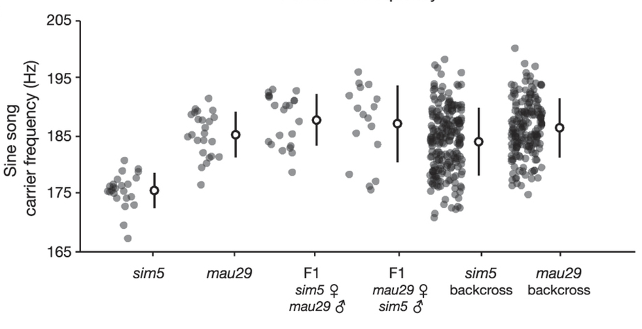
Figure 1. Sine song carrier frequency in parental strains, F1 hybrids, and backcross males.
-
their phenotype \(\{f_k\}_{k=1}^{N}\) (sine song male frequencies for our example),
-
their genotype \(\{g_k\}_{k=1}^{N}\) (using for instance RNA-seq).
We have observed that the mau allele is largely dominant (Figure 1, a reproduction of Figure 1b in Ding. et al.). For a backcrossed male fly \(k\), we use \(g_k\) to designate a sim homozygous male, that is, if the sim sequence is present in both alleles, we assign \(g_k=1\), otherwise (the mau sequence is in at least one allele) we use \(g_k=0\).
In real life, you are going to test a large number of potential informative loci, here for simplicity we consider that one single loci.
The models
-
QTL model: The loci is responsible for the phenotype such that there is a linear fit
\[f_k = a + b g_k + \epsilon,\]where the error \(\epsilon\) is drawn from a Gaussian distribution \({\cal N}(0, \sigma_Q)\).
Then, the probability of the data \(D=\{f_k,g_k\}\) given the QTL model with parameters \(a\), \(b\) and \(\sigma_Q\) is
\[P(D\mid a, b, \sigma_Q, QTL) = \frac{1}{\left(\sqrt{2\pi}\sigma_Q\right)^N} e^{-\frac{\sum_k (f_k-a-b g_k)^2}{2\sigma_Q^2}}\] -
NQTL model: the loci does not explain the phenotype (the null model),
\[f_k = c + \epsilon,\]Then, the probability of the data \(D=\{f_k,g_k\}\) given the NQTL model with parameters \(c\) and \(\sigma_{N}\) is
\[P(D\mid c, \sigma_N, NQTL) = \frac{1}{\left(\sqrt{2\pi}\sigma_N\right)^N} e^{-\frac{\sum_k (f_k-c)^2}{2\sigma_N^2}}\]
Deciding if this loci has a quantitative influence in the phenotype becomes a hypothesis testing question, that requires evaluating this quantity:
\[\frac{P(QTL\mid D)}{P(NQTL\mid D)}.\]Hypothesis testing
As we have seen before
\[\frac{P(QTL\mid D)}{P(NQTL\mid D)} = \frac{P(D\mid QTL)}{P(D\mid NQTL)}\frac{P(QTL)}{P(NQTL)} .\]Assuming we have no idea of whether the loci is or not a QTL, we use \(P(QTL) = P(NQTL) = 1/2\), then the comparison of the models becomes the comparisons of the evidences
\[\frac{P(QTL\mid D)}{P(NQTL\mid D)} = \frac{P(D\mid QTL)}{P(D\mid NQTL)} .\]For the QTL model, we have 2 parameters (\(a\) and \(b\)) for the straight line fit, and one parameter for the Gaussian noise (\(\sigma_Q\)). The NQTL model depends on 2 parameters \(c\) and \(\sigma_N\).
If we further assume that \(\sigma_Q\) and \(\sigma_N\) are known,
\[\begin{aligned} P(D\mid QTL) &= \int_{-\infty}^{\infty} da \int_{-\infty}^{\infty} db\, P(D\mid a, b, \sigma_Q, QTL)\, P(a,b\mid QTL),\\ P(D\mid NQTL) &= \int_{-\infty}^{\infty} dc\, P(D\mid c, \sigma_N, NQTL)\, P(c\mid NQTL). \end{aligned}\]The prior probability
We assume independent and flat priors,
\[P(a,b\mid QTL)=P(a\mid QTL)P(b\mid QTL),\]such that,
\[\begin{aligned} P(a\mid QTL) &= \left\{ \begin{array}{cc} \frac{1}{\sigma_a}\equiv\frac{1}{a^{+}-a^{-}} & a^{-}\leq a \leq a^{+},\\ 0 & \mbox{otherwise} \end{array} \right.\\ P(b\mid QTL) &= \left\{ \begin{array}{cc} \frac{1}{\sigma_b}\equiv\frac{1}{b^{+}-b^{-}} & b^{-}\leq b\leq b^{+},\\ 0 & \mbox{otherwise} \end{array} \right.\\ P(c\mid NQTL) &= \left\{ \begin{array}{cc} \frac{1}{\sigma_c}\equiv\frac{1}{c^{+}-c^{-}} & c^{-}\leq c\leq c^{+},\\ 0 & \mbox{otherwise} \end{array} \right. \end{aligned}\]where we have introduced,
\[\sigma_a \equiv a_{+} - a_{-} > 0,\quad \sigma_b \equiv b_{+} - b_{-} > 0,\] \[\sigma_c \equiv c_{+} - c_{-} > 0,\]for some constant values \(a_{\pm}\), \(b_{\pm}\), and \(c_{\pm}\) which are arbitrary but large enough not to introduce a cut in the evidence.
Approximating the probability of the data
Remember from w02 that you can take the ML value of the parameters and their confidence value to approximate \(P(D\mid a, b, \sigma_Q, QTL)\) and \(P(D\mid c, \sigma_N, NQTL)\).
Introducing the log probabilities
\[\begin{aligned} L^{Q}(a,b) \equiv \log P(D\mid a, b, \sigma_Q, QTL),\\ L^{N}(c) \equiv \log P(D\mid c, \sigma_N, NQTL). \end{aligned}\]A Taylor expansion around the ML values results in
\[\begin{aligned} L^{Q}(a,b) &\approx L^{Q}(a^\ast, b^\ast) +\frac{1}{2}\left.\frac{\delta^2 L^{Q}}{\delta a^2}\right|_{\ast} (a-a^\ast)^2 +\frac{1}{2}\left.\frac{\delta^2 L^{Q}}{\delta b^2}\right|_{\ast} (b-b^\ast)^2 +\left.\frac{\delta^2 L^{Q}}{\delta a\delta b}\right|_{\ast} (a-a^\ast)(b-b^\ast) \\ L^{N}(c) &\approx L^{N}(c^\ast) + \frac{1}{2}\left.\frac{\delta^2 L^{N}}{\delta c^2}\right|_{\ast} (c-c^\ast)^2 \end{aligned}\]where the ML values of the parameters \(a^\ast, b^\ast, c^\ast\) are defined by
\[\left.\frac{\delta L^{Q}}{\delta a}\right|_{\ast} = 0,\quad \left.\frac{\delta L^{Q}}{\delta b}\right|_{\ast} = 0,\] \[\left.\frac{\delta L^{N}}{\delta c}\right|_{\ast} = 0.\]The ML values of the parameters and their confidence values
Let’s calculate the actual values of the ML parameters and their confidence values.
The log probabilities are given by
\[\begin{aligned} L^Q &\propto - \frac{\sum_k (f_k-a-b g_k)^2}{2\sigma_Q^2},\\ L^N &\propto - \frac{\sum_k (f_k-c)^2}{2\sigma_N^2}, \end{aligned}\]where we are keeping only the terms that depend on the parameters we are going to optimize.
Then, the first derivatives respect to the parameters are
\[\begin{aligned} \frac{\delta L^{Q}}{\delta a} &= \frac{1}{\sigma_Q^2}\sum_k (f_k-a-b g_k),\\ \frac{\delta L^{Q}}{\delta b} &= \frac{1}{\sigma_Q^2}\sum_k (f_k-a-b g_k)g_k,\\ \frac{\delta L^{N}}{\delta c} &= \frac{1}{\sigma_N^2}\sum_k (f_k-c). \end{aligned}\]Then, introducing
\[\overline{f} = \frac{1}{N}\sum_k f_k,\quad \overline{g} = \frac{1}{N}\sum_k g_k,\] \[\overline{gg} = \frac{1}{N}\sum_k g_k g_k,\quad \overline{fg} = \frac{1}{N}\sum_k f_k g_k,\]we have for the ML values of the parameters,
\[\begin{aligned} b^\ast &= \frac{\overline{fg} - \overline{f}\overline{g}}{\overline{gg} - \bar{g}\bar{g}},\\ a^\ast &= \overline{f} - b^\ast \overline{g},\\ c^\ast &= \overline{f}.\\ \end{aligned}\]provided that \(\overline{gg} - \bar{g}\bar{g}\neq 0\).
As for the confidence values
\[\begin{aligned} \frac{\delta^2 L^{Q}}{\delta a^2} &= -\frac{N}{\sigma_Q^2} \\ \frac{\delta^2 L^{Q}}{\delta b^2} &= -\frac{N}{\sigma_Q^2}\overline{gg}, \\ \frac{\delta^2 L^{Q}}{\delta a \delta b} &= -\frac{N}{\sigma_Q^2}\overline{g}, \\ \frac{\delta^2 L^{N}}{\delta c^2} &= -\frac{N}{\sigma_N^2}. \end{aligned}\]Exponentiating the approximations to the log probabilities, we obtain the following approximations
\[\begin{aligned} P(D\mid a, b, \sigma_Q, QTL) &\approx P(D\mid a^\ast, b^\ast, \sigma_Q, QTL)\,\, \mbox{exp} \left[ +\frac{1}{2}\left.\frac{\delta^2 L^Q}{\delta a^2}\right|_{\ast} (a-a^\ast)^2 +\frac{1}{2}\left.\frac{\delta^2 L^Q}{\delta b^2}\right|_{\ast} (b-b^\ast)^2 +\left.\frac{\delta^2 L^Q}{\delta a\delta b}\right|_{\ast} (a-a^\ast)(b-b^\ast) \right]\\ P(D\mid c, \sigma_N, NQTL) &\approx P(D\mid c^\ast, \sigma_N, NQTL)\,\, \mbox{exp} \left[ +\frac{1}{2}\left.\frac{\delta^2 L^N}{\delta c^2}\right|_{\ast} (c-c^\ast)^2 \right]. \end{aligned}\]Putting things together
Introducing the \(2\times 2\) matrix \(Q\)
\[Q = \frac{N}{\sigma_Q^2} \left( \begin{array}{cc} 1 & \overline{g}\\ {\overline g} & \overline{gg} \end{array} \right)\]then we can write
\[\begin{aligned} P(D\mid QTL) &\approx P(D\mid a^\ast, b^\ast, \sigma_Q, QTL)\, \left[ \int da \int db\, e^{-\frac{1}{2}(a-a^\ast,b-b^\ast) Q {a-a^\ast\choose b-b^\ast}} \right]\, \frac{1}{\sigma_a}\frac{1}{\sigma_b} \\ P(D\mid NQTL) &\approx P(D\mid c^\ast, \sigma_N, NQTL)\, \left[ \int dc\, e^{-\frac{1}{2}\frac{N}{\sigma_N^2}(c-c^\ast)^2} \right]\, \frac{1}{\sigma_c} . \end{aligned}\]These integrals can be approximated by a closed form expression (the case of the NQTL model with one parameter we did explicitly in w03).
we have,
\[\begin{aligned} P(D\mid QTL) &\approx P(D\mid a^\ast, b^\ast, \sigma_Q, QTL) \times \frac{2\pi}{\sqrt{\det{Q}}}\frac{1}{\sigma_a \sigma_b}\, \\ P(D\mid NQTL) &\approx P(D\mid c^\ast, \sigma_N, NQTL) \times \sqrt{\frac{2\pi\sigma_N^2}{N}}\frac{1}{\sigma_c}. \end{aligned}\]Finally!
The ratio of the probabilities of the QTL respect to the NQTL model is given by
\[\frac{P(QTL\mid D)}{P(NQTL\mid D)} = \frac{P(D\mid a^\ast, b^\ast, \sigma_Q, QTL)}{P(D\mid c^\ast, \sigma_N, NQTL)} \times \sqrt{\frac{2\pi/N}{\overline{gg} - \bar{g} \bar{g}}} \frac{ \frac{\sigma_Q}{\sigma_a}\frac{\sigma_Q}{\sigma_b} } { \frac{\sigma_N}{\sigma_c} } .\]Notice the presence of both the data fit term and the Occam’s razor term. The QTL includes the NQTL model as a particular case, so by looking at the data fit term, the QTL model would always have higher probability than the NQTL model. It is the Occam’s razor term the one that compensates by the fact that the QTL model has one more parameter than the NQTL model.
In Ding et. al, they use a method similar to Lander & Botstein, in which they only calculate the data fit term (named LOD). All LOD are always positive (see Lander/Botstein, Figures 2 and 3). Thus, they need to find threshold values (named T), “above which a QTL will be declared present”. Selecting the appropriate threshold T is “an important issue […] What LOD threshold T should be used in order to maintain an acceptably low rate of false positives?”.
Identifying the threshold(s) T becomes a classical p-value calculation based on additional experiments for some previously known true and false QTLs. Besides, different thresholds have to be apply depending on the genome size and the density of restriction enzyme marks (see Lander/Botsein, Figure 4).
Doing the proper Bayesian calculation removes the need for such threshold value.
Generalization to many loci
If we are trying to test if the observed phenotype variability is do to more than one loci, we would include one parameter \(b^\alpha\) for each locus tested \(1\leq \alpha\leq L\) as
\[f_k = a + \sum_{\alpha = 1}^{L} b^\alpha g^\alpha_k + \epsilon.\]Assumptions
These are the assumptions in the QTL mapping derivation presented here, each of which could be questioned and removed if necessary
-
Linear fit between phenotype and genotype.
-
Gaussian noise.
-
All noise follows the same Gaussian \({\cal N}(0, \sigma)\),
-
\(\sigma\) is known.
-
For the linear regression parameters, we have integrated their posterior probability approximated by a second-order Taylor expansion of the log probability around their maximum likelihood values.