MCB111: Mathematics in Biology (Fall 2024)
- The biological example
- Why you want to optimize the parameters
- Maximum likelihood: parameter estimation for complete data
- Expectation Maximization: parameter estimation for incomplete data
- Why does Expectation-Maximization work?
week 07:
Probabilistic models and Expectation Maximization
In this lecture, we are going to investigate the problem of training a probabilistic graphical model or Bayesian network. We will describe the method of Maximum likelihood used when we have completely annotated data, and the method of Expectation-Maximization used when the available data for training is incompletely labeled.
For this week’s lectures, if you do not read anything else, I recommend the article “What is the expectation maximization algorithm?” by Do & Batzoglou.
I am going to rephrase the contents of that article using our example of the HMM model described by Andolfatto et al. to assign ancestry to chromosomal segments.
The biological example
We are continuing with the biological problem that we introduced in week06. Andolfatto et al. introduced an HMM to assign ancestry to male fly backcrosses for which we know the genomic sequence, and have mapped reads for each backcross individual.
The experimental design allows two ancestral states \(Z=\{AB, BB\}\)
-
Heterozygous for Drosophila Simulans (A=Dsim) and Drosophila Sechellia (B=Dsec)
\[Z = AB\] -
Homozygous for Drosophila Sechellia (B=Dsec)
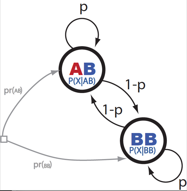
Figure 1. The ancestry HMM.
The HMM is described in Figure 1. The transition probabilities from being at ancestry \(Z_i\) at locus \(i\) given the ancestry at the previous locus \(Z_{i-1}\) are parameterized by one Bernoulli parameter \(p\),
\[P(Z_i\mid Z_{i-1}) = \left\{ \begin{array}{cc} p & \mbox{for}\ Z_i = Z_{i-1}\\ 1-p & \mbox{for}\ Z_i \neq Z_{i-1} \end{array} \right.\]In their paper, Andolfatto et al. assigned the value of \(p\), based what it is already known about recombination in Drosophila species. Mainly, that one should expected on average one recombination event from chromosome. That means that in some individuals you will find one, in others 0, in others 2, maybe a few rare cases with three or more, such that the average will be close to one.
If there is on average one break per chromosome, then the average length of a region without breakpoints should be \(L/2\) for a chromosome of length \(L\), and because the mean of a geometric distribution of Bernoulli parameter \(p\) is \(p/(1-p)\), that determines the parameter to take the value
\[p = \frac{L/2}{L/2+1}.\]For some real numbers in Drosophila,
- Chromosome 2L, length = 23.01 million bases
- Chromosome 4, is much shorter length = 1.35 million bases
Does such small difference in the values of \(p\) make any difference in the inference results?
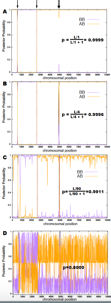
Figure 2. Analysis of a chromosomal fragment with 4 breakpoints indicated on top with an arrow. Posterior probabilities identifying the breakpoints are depicted for three different values of the Bernoulli parameter for the HMM, p: (A) Assumes that one breakpoint is expected. (B) Assumes 4 breakpoints (the actual number in the segment). (C) Assumes that 90 breaks are expected. (D) The Bernoulli parameter is set to 0.8 , which should produce on average 2,500 breakpoints.
Why you want to optimize the parameters
Let’s now concentrate in our re-implementation of the Andolfatto HMM which we did last week. Because our implementation uses some slow scripting programming language (python, perl, matlab…), we probably cannot deal with very long sequences, so let’s assume a chromosome of length \(L=10,000\).
Because this is a generative model, I have the advantage that I can generate the data what otherwise you will have to painfully collect in your experiments. For this example, I have introduced 4 breakpoints.
I ran the decoding algorithm of week 06, for four different values of the Bernoulli parameter, that correspond to a expected number of breakpoints of \(1, 4, 90, 2500\) respectively. Results are given in Figure 2.
Panel (B) corresponds to the optimal value of \(p\), which identifies the 4 breakpoints, and only those breakpoints. In panel (A), a value of \(p\) the would result in fewer expected breakpoints, misses two of them, the two that are very closed together. In panel (C) you observe how as your parameter lowers the number of predicted breakpoints (false positives) increases. Finally, panel (D) shows how sensitive the results are to changes in the value of the parameters.
So, if you are now convinced that the value of the parameters matter, sometimes when the differences are tiny, how do we obtain the optimal value of the parameters?
Maximum likelihood: parameter estimation for complete data
In many cases, you have a number of examples in which the data is actually labeled. In our case, that would mean, a collection individuals (male flies) with mapped reads for which we know the ancestry for all loci (see Figure 3). We call this data set of labeled data the training set.
Using the training set, you can calculate the number of times (counts) that each possible transition occurs at each locus \(i\),
\[C_i(AB\rightarrow AB)\\ C_i(BB\rightarrow BB)\\ C_i(AB\rightarrow BB)\\ C_i(BB\rightarrow AB).\]After collecting all the counts for all loci \(i\) and for all individuals \(1\leq m \leq M\), we can calculate the frequency of the parameter \(p\) as
\[p = \frac{\sum_m\sum_i C^m_i(AB\rightarrow AB) + \sum_m\sum_i C^m_i(BB\rightarrow BB)} {[\sum_m\sum_i C^m_i(AB\rightarrow AB)+\sum_m\sum_i C^m_i(BB\rightarrow BB)]+[\sum_m\sum_i C^m_i(AB\rightarrow BB)+\sum_m\sum_i C^m_i(BB\rightarrow AB)]}\]This intuitive estimation of the value of the parameters is called the maximum likelihood estimation.
The reason is because those estimates are the value of the parameters that maximize the probability of the data in the training set.
Maximum likelihood derivation
In order to apply ML, we need to have a set of \(M\) individuals for which we know both the reads and the ancestry for a given genomic loci of length \(L\). That is, the data is
\[D = \{(X^1_1 Z^1_1,\ldots,X^1_L Z^1_L),\ldots ,(X^M_1 Z^M_1,\ldots,X^M_L Z^M_L)\}.\]The probability of the data, given the model that depends on the parameters \(p\) is
\[P(D\mid p) = \prod_{m=1}^M P(X^m_1\ldots X^m_L\mid p).\]Introducing the log probability \(L^m(X^m_1\ldots X^m_L\mid p) = \log P(X^m_1\ldots X^m_L\mid p)\), the log probability of the data \(D\) given the parameter \(p\) is given by
\[L(D\mid p) = \log P(D\mid p) = \sum_{i=1}^M L^m(X^m_1\ldots X^m_L\mid p).\]The ML value of the parameter named \(p^\ast\), is given by
\[\left.\frac{d L(X^m_1\ldots X^m_L)}{d p}\right|_{p^\ast} = 0.\]Notice that under uniform prior hypothesis for \(p\), the ML value, \(p\ast\), is also the value that maximizes the posterior probability of the parameter \(p\).
We all generality, we can write
\[P(D\mid p) = \prod_{m=1}^M\prod_{i=1}^L p^{C^m_i(BB\rightarrow BB) + C^m_i(AB\rightarrow AB)}(1-p)^{C^m_i(BB\rightarrow AB) + C^m_i(AB\rightarrow BB)}.\]Then
\[L(D\mid p) = \log(p) \sum_m\sum_i C^m_i(BB\rightarrow BB) + C^m_i(AB\rightarrow AB) + \log(1-p) \sum_m\sum_i C^m_i(BB\rightarrow AB) + C^m_i(AB\rightarrow BB).\]The derivative respect to \(p\), is given by
\[\frac{d L(D\mid p)}{d p} = \frac{1}{p} \sum_m\sum_i \left[C^m_i(BB\rightarrow BB) + C^m_i(AB\rightarrow AB)\right] - \frac{1}{1-p}\sum_m\sum_i \left[C^m_i(BB\rightarrow AB) + C^m_i(AB\rightarrow BB)\right].\]The ML condition results in
\[\frac{1}{p^\ast} \sum_m\sum_i \left[C^m_i(BB\rightarrow BB) + C^m_i(AB\rightarrow AB)\right] = \frac{1}{1-p^\ast}\sum_m\sum_i \left[C^m_i(BB\rightarrow AB) + C^m_i(AB\rightarrow BB)\right].\]That is, the expression we proposed above
\[p^\ast = \frac{\sum_m\sum_i\left[ C^m_i(AB\rightarrow AB) + C^m_i(BB\rightarrow BB)\right]} {\sum_m\sum_i \left[\ C^m_i(AB\rightarrow AB) + C^m_i(BB\rightarrow BB)\right] + \sum_m\sum_i \left[\ C^m_i(AB\rightarrow BB) + C^m_i(BB\rightarrow AB)\right]}\]This results generalizes when there is more than one parameters. If the transition from ancestry \(AB\) could have \(k\) possible values \(p(Z_k\mid AB)\), such that \(\sum_k P(Z_k\mid AB) = 1\), the ML estimate from labeled data is given by the the fraction of the number of times that the transition \(AB\rightarrow Z_k\) occurs in the data (\(n(AB\rightarrow Z_k)\)),
\[P(Z_k\mid AB) = \frac{n(AB\rightarrow Z_k)}{\sum_{k^\prime} n(AB\rightarrow Z_{k^\prime})}.\]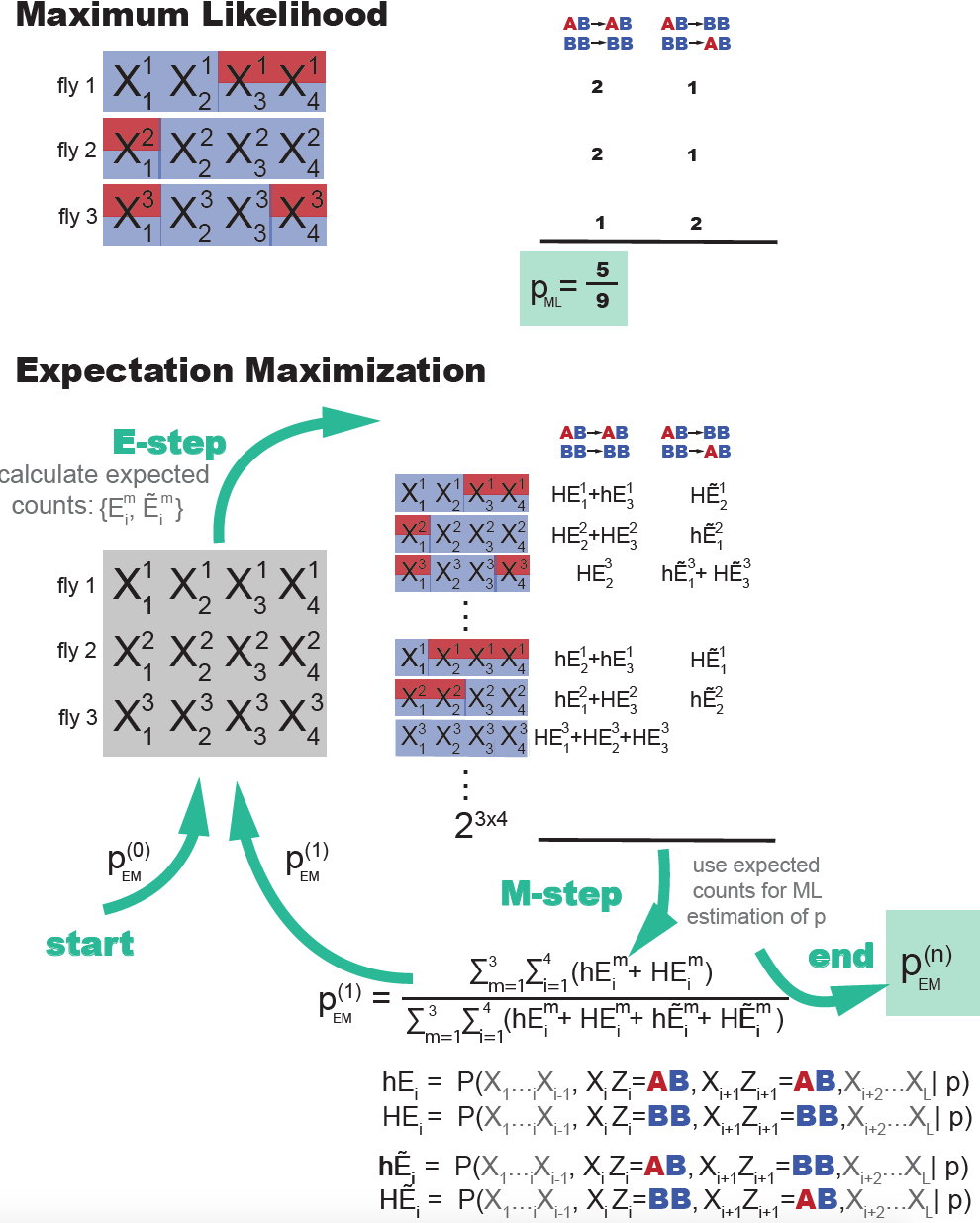
Figure 3. A re-implementation of Do & Batzoglou's Figure 1 comparing Maximum likelihood training in the presence of labeled data, versus Expectation Maximization training when the data is not labeled. In ML estimation, the parameters are given by their frequency in the training set. In EM estimation, there is an iterative process. At each EM cycle, all possible labelings of the data are considered each weighted by their expected counts (the E-step). Using all those expected counts new ML parameters are estimated. The recursion ends when parameters converge.
Expectation Maximization: parameter estimation for incomplete data
But most of the time, we do not have labeled data, you may have mapped reads for many different male flies, but not the corresponding labeling of the ancestry.
In this situation, you can use a iterative method named Expectation Maximization EM). For the particular example of an HMM, as it is our case here, it also goes by the name of the Baum-Welch algorithm.
The EM algorithm has the following steps (Figure 3)
-
start
One starts with some arbitrary value of the parameters.
For our case with one parameter
\[p^{(0)}.\] -
E-step (expectation)
In this step you calculate the expected number of times each of the transitions is used in each locus, assuming that you sum to all other possible values of the ancestry for all other loci. That is
\[\begin{aligned} E_i(AB\rightarrow AB) &= P(X_i\ldots X_{i-1}, X_i Z_i = AB, X_{i+1} Z_{i+1} = AB, X_{i+2}\ldots X_{L}\mid p^{(0)})\\ E_i(BB\rightarrow BB) &= P(X_i\ldots X_{i-1}, X_i Z_i = BB, X_{i+1} Z_{i+1} = BB, X_{i+2}\ldots X_{L}\mid p^{(0)})\\ E_i(AB\rightarrow BB) &= P(X_i\ldots X_{i-1}, X_i Z_i = AB, X_{i+1} Z_{i+1} = BB, X_{i+2}\ldots X_{L}\mid p^{(0)})\\ E_i(BB\rightarrow AB) &= P(X_i\ldots X_{i-1}, X_i Z_i = BB, X_{i+1} Z_{i+1} = AB, X_{i+2}\ldots X_{L}\mid p^{(0)})\\ \end{aligned}\]These expected counts are the equivalent of the counts in the case of having labeled data.
The expected counts are easily calculated from the forward and backward probabilities calculated using the forward and backward algorithms introduced in week 06 for each individual \(m\),
\[\begin{aligned} E^m_i(AB\rightarrow AB) &= f_{i,m}^{AB}\ p^{(0)}\ P(X^m_{i+1}\mid AB)\ b_{i+1,m}^{AB}\\ E^m_i(BB\rightarrow BB) &= f_{i,m}^{BB}\ p^{(0)}\ P(X^m_{i+1}\mid BB)\ b_{i+1,m}^{BB}\\ E^m_i(AB\rightarrow BB) &= f_{i,m}^{AB}\ (1-p^{(0)})\ P(X^m_{i+1}\mid BB)\ b_{i+1,m}^{BB}\\ E^m_i(BB\rightarrow AB) &= f_{i,m}^{BB}\ (1-p^{(0)})\ P(X^m_{i+1}\mid AB)\ b_{i+1,m}^{AB}\\ \end{aligned}\] -
M-step (maximization)
\[p^{(1)} = \frac{\sum_m\sum_i E^m_i(AB\rightarrow AB) + \sum_m\sum_i E^m_i(BB\rightarrow BB)} {[\sum_m\sum_i E^m_i(AB\rightarrow AB)+\sum_m\sum_i E^m_i(BB\rightarrow BB)]+[\sum_m\sum_i E^m_i(AB\rightarrow BB)+\sum_m\sum_i E^m_i(BB\rightarrow AB)]}\]The new \(p^{(1)}\) are used for a new round of the E-step
-
end
We iterate the E-step/M-step until convergence, that is \(p^{(n)} \approx p^{(n+1)}\).
EM optimization of other conditional probabilities
We could also use the EM algorithm to optimize the conditional probabilities \(P(X\mid AB)\) and \(P(X \mid BB)\).
We can introduce,
\[\begin{aligned} E_i(X\mid AB) = E_{i-1}(AB\rightarrow AB)+E_{i-1}(BB\rightarrow AB) &= P(X_{i}=X\mid AB)\ \left[ \ p^{(0)}\ f_{i-1}^{AB}\ b_{i}^{AB} + \ (1-p^{(0)})\ f_{i-1}^{BB}\ b_{i}^{AB}\right]\\ E_i(X\mid BB) = E_{i-1}(BB\rightarrow BB)+E_{i-1}(AB\rightarrow BB) &= P(X_{i}=X\mid BB)\ \left[ \ p^{(0)}\ f_{i-1}^{BB}\ b_{i}^{BB} + \ (1-p^{(0)})\ f_{i-1}^{AB}\ b_{i}^{BB}\right]. \end{aligned}\]Then, the EM algorithm for optimizing \(P(X\mid AB)\) and \(P(X \mid BB)\) is as,
-
E-step (expectation)
Calculate the expected values
\[\begin{aligned} E^m_i(X\mid AB) &= P^{(0)}(X^m_{i}=X\mid AB)\ \left[ \ p^{(0)}\ f_{i-1,m}^{AB}\ b_{i,m}^{AB} + \ (1-p^{(0)})\ f_{i-1,m}^{BB}\ b_{i,m}^{AB}\right] \\ E^m_i(X\mid BB) &= P^{(0)}(X^m_{i}=X\mid BB)\ \left[ \ p^{(0)}\ f_{i-1,m}^{BB}\ b_{i,m}^{BB} + \ (1-p^{(0)})\ f_{i-1,m}^{AB}\ b_{i,m}^{BB}\right]. \end{aligned}\] -
M-step (maximization)
Update \(P(X\mid AB)\) and \(P(X \mid BB)\) as follows
\[\begin{aligned} P^{(1)}(X\mid AB) &= \frac{\sum_i\sum_m E^m_{i}(X\mid AB) } {\sum_{X}\sum_i\sum_m\ E^m_{i}(X\mid AB)} \\ P^{(1)}(X\mid BB) &= \frac{\sum_i\sum_m\ E^m_{i}(X\mid BB)} {\sum_X \sum_i\sum_m\ E^m_{i}(X\mid BB)}. \end{aligned}\]
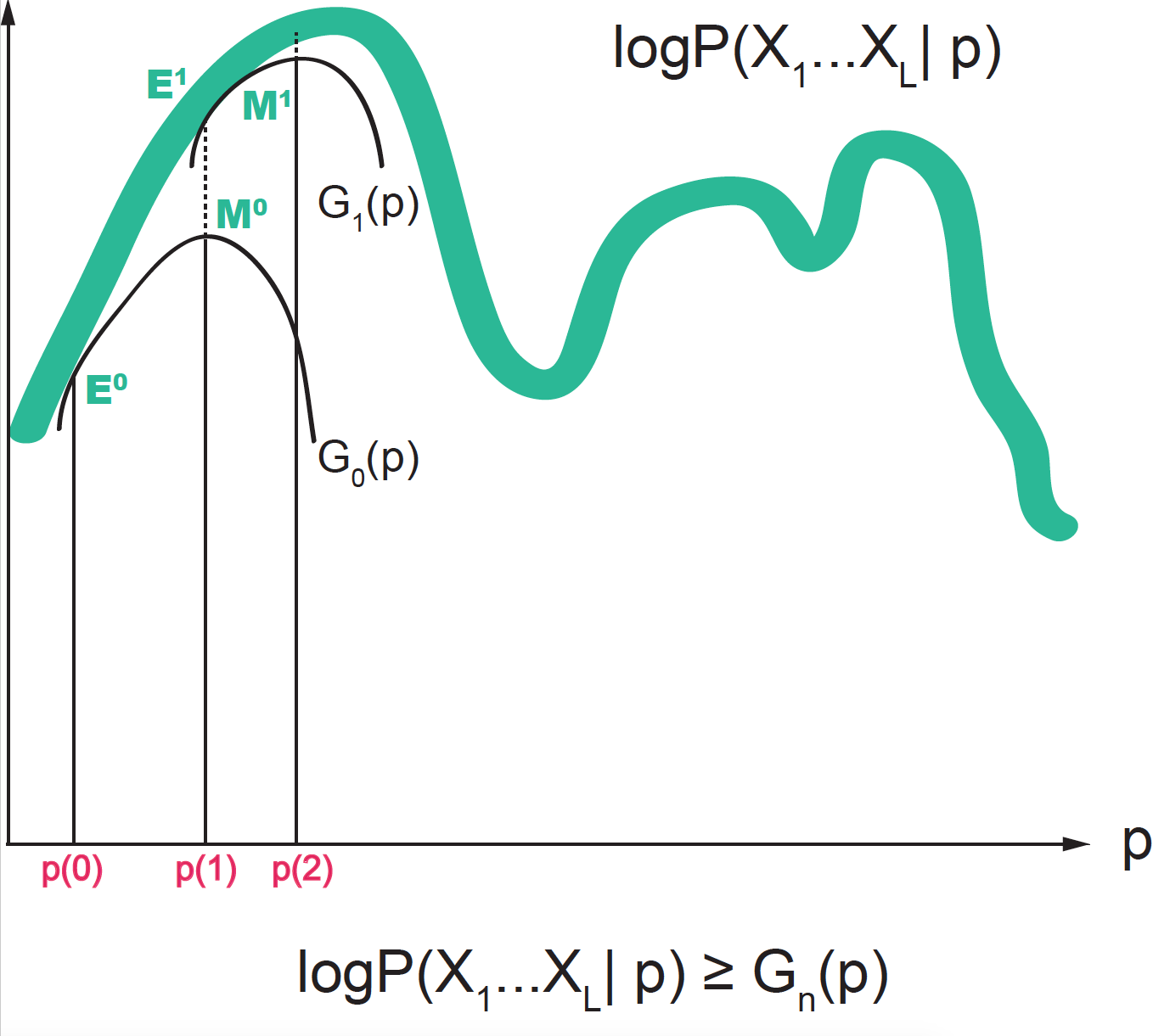
Figure 4. The probability distribution is approximated at each step (n) by a function G(n) guaranteed to be a lower bound for the actual distribution. In the E-step, we use the current value of the parameters to find the "expected values". In the M-step, we use those expectations in order to find new values for the parameters that optimize the lower bound function G(n).
Why does Expectation-Maximization work?
A graphical description of how EM works
In the EM algorithm, we alternate between two actions, see Figure 4.
-
In the E-step, given a set of values for the parameters, we obtain expected counts for al possible labels.
-
In the M-step, we use those expected counts to obtain new estimations for the parameters. The M-step can be justified as the new values of the parameters are the maximum-likelihood values for a function related to our full probability distribution by being a lower bound.
EM as a Variational Method
The EM algorithm belongs to the class of variant methods in which the optimal value for a function as calculated using a different but related (variational) objective function.
Let’s use
\[D = \{X^m_1\ldots X^m_L\}_{m=1}^M\]to describe the observed data (in out case the collection of mapped reads for all loci for all male backcross flies).
Let’s use
\[Z = \{Z^m_1\ldots Z^m_L\}_{m=1}^M\]to refer to the unobserved lated data (in our case the ancestry for all loci for all male backcross flies).
And let’s use \(p\) to refer to a vector of unknown parameters (in our case just one)
\[p = P(AB\mid AB) = P(BB\mid BB).\]We can always write by marginalization, for \(z\in Z\)
\[P(D\mid p) = \sum_{z\in Z} P(D, z\mid p).\]For any arbitrary probability distribution on the unobserved data \(Q(z)\)
\[\log P(D\mid p) =\log \sum_z P(D, z\mid p) = \log \sum_z Q(z)\frac{P(D, z\mid p)}{Q(z)}\]such that \(Q(z)\) is a probability distribution in \(Z\), that is \(\sum_z Q(z) = 1\). The variant distribution \(Q\) could also be conditioned on the data \(X\) or even a completely different set of parameters \(\theta\)!, but not on the parameters \(p\) that we are trying to optimize.
Using Jensen’s inequality, we can write
\[\log P(D\mid p) \geq \sum_z Q(z\mid D) \log \frac{P(D, z\mid p)}{Q(z\mid D)}.\]Then two expressions become equal for \(Q(z\mid D) = P(z\mid D, p)\).
In the EM algorithm, we are going to select a different variant distribution for each iteration \(n\), where the parameters take values \(p^{(n)}\)
\[Q_{n}(z\mid D) = P(z\mid D, p^{(n)})\]Notice that these variant distribution is exactly the quantities \(E\) that we calculate in the E-step of each iteration.
Introduce
\[G_n(D\mid p) = \sum_z P(z\mid D, p^{(n)}) \log \frac{P(D, z\mid p)}{P(z\mid D, p^{(n)})}\]Then
\[\log P(D\mid p) \geq G_n(D\mid p)\]Then
\[argmax_p \log P(D\mid p) \geq argmax_p G_n(D\mid p)\]and maximizing \(G_n(D\mid p)\) one each iteration results in a improvement for \(\log P(D\mid p).\)
In summary, EM consists of optimizing the function
\[logP(D\mid p)\]by optimizing at each EM iteration the variant function
\[G_n(D\mid p) = \sum_z P(z\mid D, p^{(n)}) \log \frac{P(D, z\mid p)}{P(z\mid D, p^{(n)})}\]which has the following properties (see Figure 4)
-
The variant function is a lower bound to the actual function we want to optimize:
\[G_n(D\mid p) \leq \log P(D\mid p)\] -
The two functions take the same value when the parameters are set to the current estimate \(p^{(n)}\):
\[G_n(D\mid p=p^{(n)}) = \log P(D\mid p=p^{(n)})\] -
In addition, optimizing \(G_n(D\mid p)\) is equivalent to optimizing the function:
\[argmax_p G_n(D\mid p) = argmax_p \sum_z P(z\mid D, p^{(n)}) \log P(D, z\mid p)\]as the term \(-\sum_z P(z\mid D, p^{(n)}) \log P(z\mid D, p^{(n)})\) is independent of the parameters.
Thus, at each iteration in the EM algorithm:
-
E-step
Calculate the \(P(z\mid D, p^{(n)})\) for all possible realizations of the unobserved variables.
In our particular example, we calculate the \(E^m_{i}(AB\rightarrow AB\mid p^{(n)})\), \(E^m_{i}(AB\rightarrow BB\mid p^{(n)})\), \(E^m_{i}(BB\rightarrow AB\mid p^{(n)})\), and \(E^m_{i}(BB\rightarrow BB\mid p^{(n)})\).
-
M-step
Optimize in \(p\) \(\sum_z P(z\mid D, p^{(n)}) \log P(D, z\mid p)\), that is the probability of the date \(D\) for each possible completion of the unobserved data, each completions weighted by its corresponding posterior probabilities.
A similar proof can be found in the supplemental materials of Do & Batzoglou.
The EM algorithm is guarantee to find local maxima. You would like to re-start the algorithm from different starting points and compare results.