MCB111: Mathematics in Biology (Fall 2024)
- A synthetic toggle switch in E. coli
- A synthetic oscillator in E. coli
- Molecular bases of a circadian rhythm in Drosophila
week 12:
Genetic Switches
In these lectures, we are going to discuss three different networks of interacting biomolecules. Two of them are not part of any naturally occurring system, but both have been synthetically designed in E. coli. Those are: a toggle switch with two mutually repressing molecules that produce bistability “Construction of the genetic toggle switch in E. coli.” by Gardner et al, and an oscillator named the repressilator “A synthetic oscillatory network of transcriptional regulators” by Elowitz & Leibler.
The third system is a mathematical modeling of a circadian rhythm found in Drosophila “A model for circadian oscillations in the Drosophila Period protein (PER)” by A. Goldbeter. An interesting resource about circadian rhythms comes from the Howard Hughes Medical Institute BioInteractive pages. Some more information about oscillatory systems in biology can be found in “Biomedical oscillations” by J. Tyson.
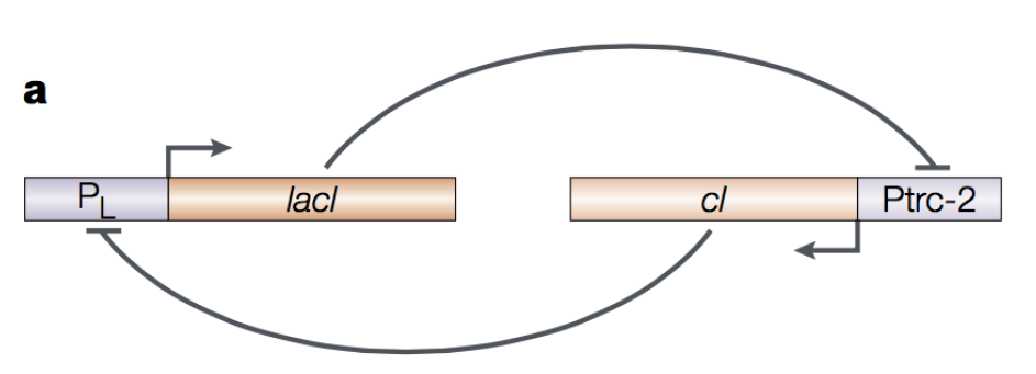
Figure 1. E. coli toggle switch. Figure by Hasty et al., Nat. Rev. Gen. 2001.
A synthetic toggle switch in E. coli
An E. coli toggle switch has been synthesized “Construction of the genetic toggle switch in E. coli.” by Gardner et al.
The E. coli toggle switch described in Figures 1 and 2, includes two transcription factors lacI and cI that inhibit each other in a double negative feedback loop that results in an overall positive feedback loop. A GFP reporter has been added to the system, such that high concentrations of cI will result in green fluorescence.
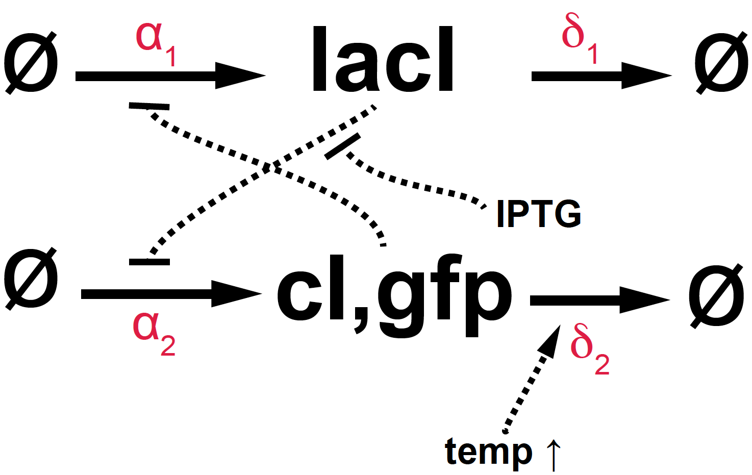
Figure 2. Diagram of the E. coli toggle switch.
This is the actual plasmid construct that was implemented
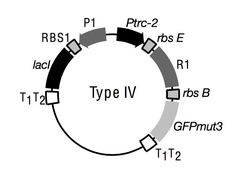
Figure 3 from Gradner et al., Nature 403, 2000. Promoters are boxes with arrows. T1/T2 are terminators. R1 generically represents a repressor gene (cI in our case). RSB are ribosomal binding sites.
The toggle system can be manipulated in two different ways:
-
Adding IPTG (Isopropyl \(\beta\)-D-1-triogalactopyranoside), a molecule that inhibits lacI, thus reducing the negative control of lacI over cI. Thus, high concentrations of IPTG would result in more green fluorescence.
-
Raising the temperature. The gene cI is a temperature mutant, such that as the temperature increases, cI degrades faster (\(\delta_2\) increases). Thus, a temperature spike should result in lower fluorescence.
Introducing the notation
\[\begin{aligned} U &= lacI\\ V &= cI, gfp\\ I &= IPTG \end{aligned}\]The kinetic equations of the E. coli switch are given by
\[\begin{aligned} \frac{d U}{d t} &= \alpha_1 \frac{K^n}{K^n+V^n} - \delta_1 U\\ \frac{d V}{d t} &= \alpha_2 \frac{K^n}{K^n+U^n} - \delta_2 V\\ \end{aligned}\]where we have introduced one Hill coefficient \(n\), and parameter \(K\) to describe both negative feedback loops. \(\alpha_1\) and \(\alpha_2\) are compound parameters that take into account both the mechanics of transcription and translation. \(\delta_1\) and \(\delta_2\) take into account the effects of degradation and dissipation.
Adding the inhibitor IPTG would results in a modification of the kinetic equation of V=cI,gfp as
\[\begin{aligned} \frac{d V}{d t} &= \alpha_2 \frac{K^n}{K^n+\left(\frac{U}{(1+I/K_m)^m}\right)^n} - \delta_2 V\\ \end{aligned}\]where another Hill coefficient \(m\), and parameter \(K_m\) has been introduced.
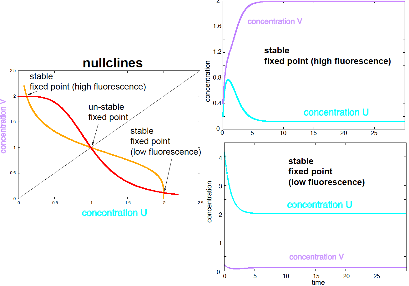
Figure 3. Nullclines and two stable fixed points. Parameters are a1 =a2 =2, d1=d2=1,n=4,K=1.
Bistability
A double negative feedback loop (as we already saw in a previous homework) results in a system with bistability. The conditions for bistability are
- High connectivity \(n >1\).
- The \(\alpha_1\) and \(\alpha_2\) parameters have similar magnitude.
- The degradation parameters \(\delta_1\) and \(\delta_2\) have similar magnitude.
- Only moderate inhibition by IPTG.
Using parameters \(\alpha_1=\alpha_2 = 2\), \(\delta_1=\delta_2 = 1\), \(n=4\), \(K=1\), the study of the nullclines tells us that the system has 3 fixed points, two of them stable (Figure 3). Of the two stable fixed points, one corresponds to high concentrations of cI and GFP, thus high fluorescence, that the other one corresponds to high concentrations lacI and low fluorescence. Using two different initial conditions, we can reach each of the two stable steady states (or fixed points), see Figure 3.
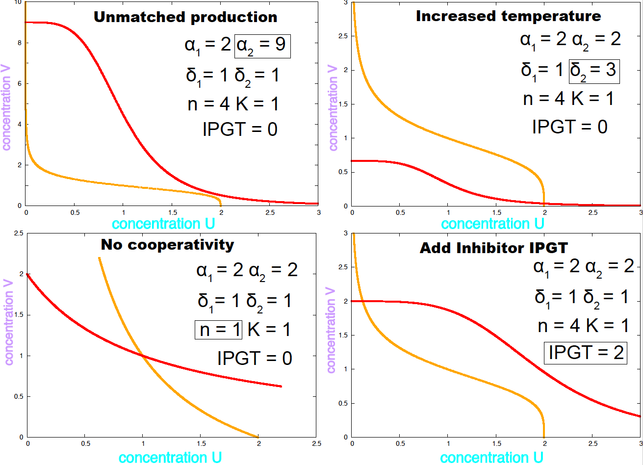
Figure 4. Examples of conditions under which the E. coli toggle becomes mono stable.
If the two \(\alpha\) parameters or the two \(\delta\) parameters have very different magnitudes, the system has only one steady state. The same happens if the Hill coefficient is \(n=1\), that is no cooperativity. Figure 4 shows the nullclines under conditions that remove bistability. Different values of the parameters result on the system changing the number of steady states, that phenomenon is called a bifurcation.
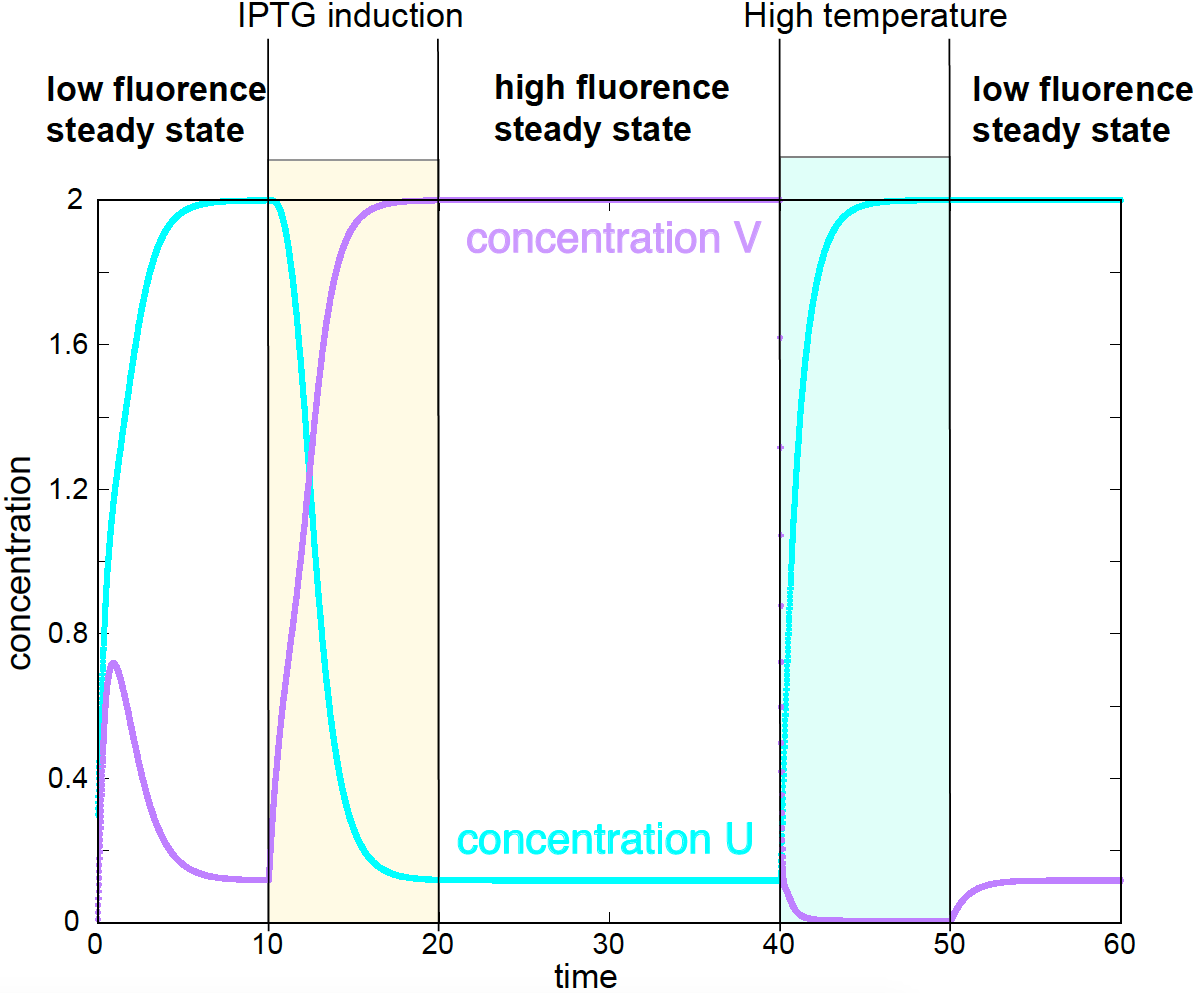
Figure 5. Theoretical switch between the two stable steady states induced by either adding an inhibitor (IPTG) or by raising the temperature. Corresponding experimental data in Figures 4, and 5 of Gardner et al.
One interesting result of this work is that they made the system switch from one steady state (high fluorescence) to another (low fluorescence) by using an inhibitor of lacI, and by raising the temperature, which increases the clearance rate of cI, see Figure 5.
For a system in the low steady state, a pulse of IPTG is added between times 10 and 20. After the inhibitor is removed at time 20, the system remains in the high steady state. At time 40, the temperature is raised which brings the system to the low steady state. After the temperature is brought back to normal at time 50, the system remains in the low steady state. Those theoretical predictions were well confirmed experimentally, see Figure 4 and 5 in Gardner et al.
A synthetic oscillator in E. coli
In “A synthetic oscillatory network of transcriptional regulators” by Elowitz & Leibler, constructed a synthetic oscillator in E. coli that then named the repressilator. Although imperfect, this is a seminal work.
The repressilator uses three transcription factors (TF) that form a negative feedback loop in which one TF inhibits the production of the next TF in a cyclic way (see Figure 6). The repressilator uses two of the same TFs used for the toggle (lacI and cI), but there is a third TF (TetR) that is placed in between the two.
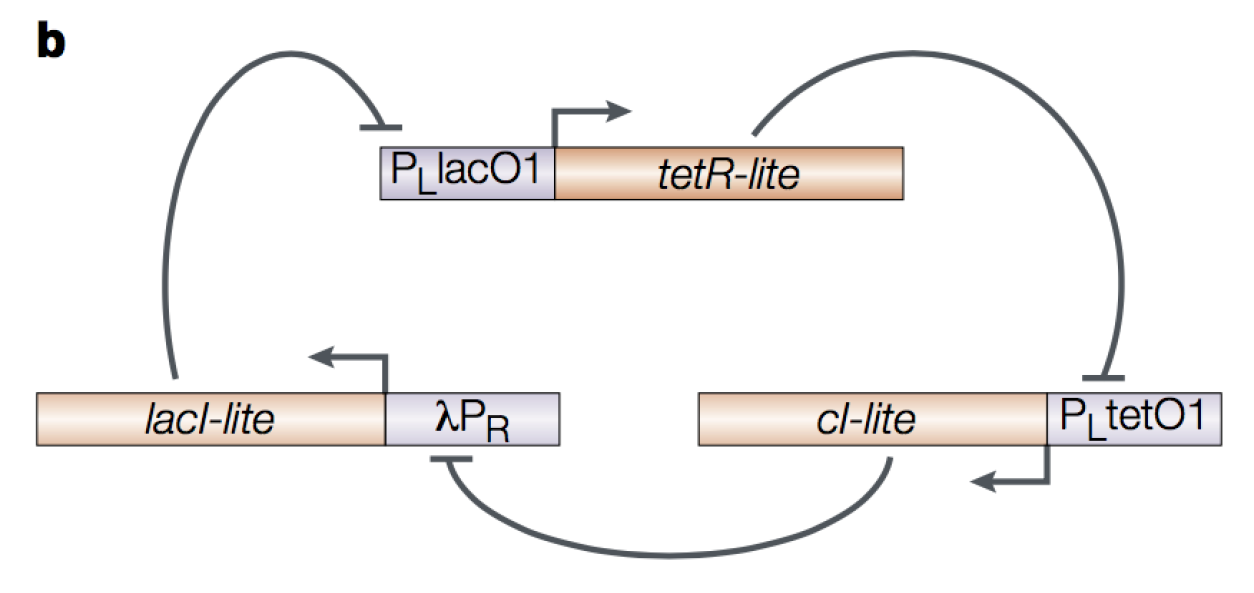
Figure 6. The E. coli repressilator. Figure by Hasty et al., Nat. Rev. Gen. 2001.
The diagrammatic representation of the repressilator is given in Figure 7. The output of the repressilator is given by a GFP reporter driven by the same promoter as cI, thus inhibited by TetR.
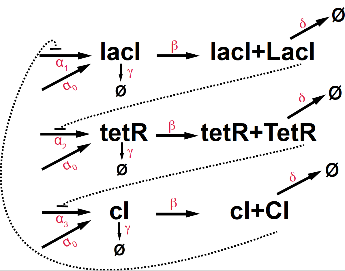
Figure 7. Kinetic diagram of the E.coli repressilator.
This is the actual construct that was implemented
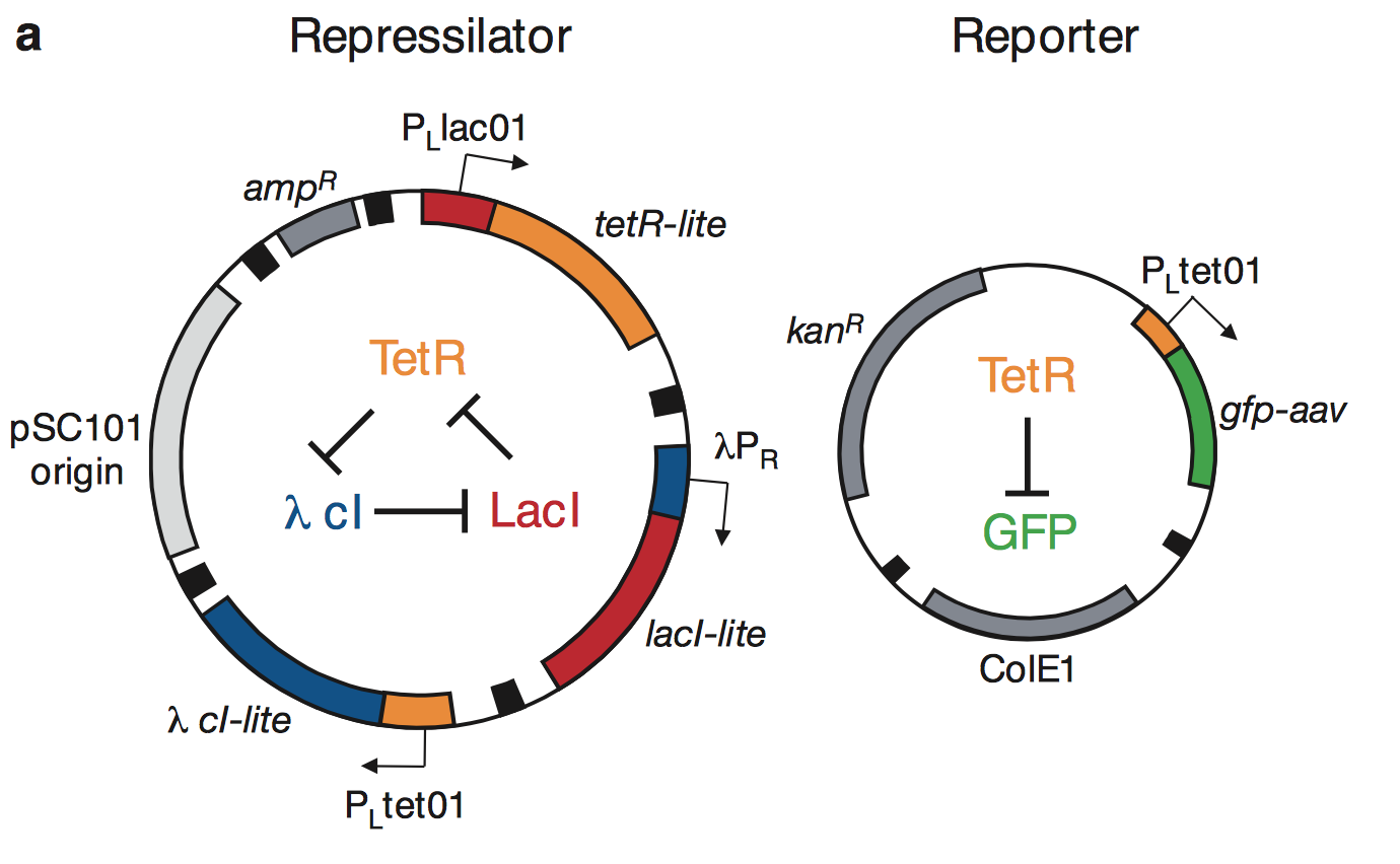
Figure 1a from Elowitz & Liebler, Nature 1999.
Introducing the notation
\[\begin{aligned} \mbox{gene}\quad &\quad \mbox{protein}\\ m1 = lacI\quad &\quad p1 = LacI\\ m2 = tetR\quad &\quad p2 = TetT\\ m3 = cI\quad &\quad p3 = CI \end{aligned}\]The kinetic equations of the E. coli repressilator are given by
\[\begin{aligned} \frac{d m_1}{d t} &= \alpha_0 + \alpha_1 \frac{K^n}{K^n+p_3^n} - \gamma m_1\\ \frac{d m_2}{d t} &= \alpha_0 + \alpha_2 \frac{K^n}{K^n+p_1^n} - \gamma m_2\\ \frac{d m_3}{d t} &= \alpha_0 + \alpha_3 \frac{K^n}{K^n+p_2^n} - \gamma m_3\\ \frac{d p_1}{d t} &= \beta m_1 - \delta p_1\\ \frac{d p_2}{d t} &= \beta m_2 - \delta p_2\\ \frac{d p_3}{d t} &= \beta m_3 - \delta p_3\\ \end{aligned}\]Oscillations
Using numerical simulations, we can determine the value of the parameters under which the repressilator observes oscillations. Here is a typical set of parameters under which there is not one stable steady state but oscillations (Figure 8).
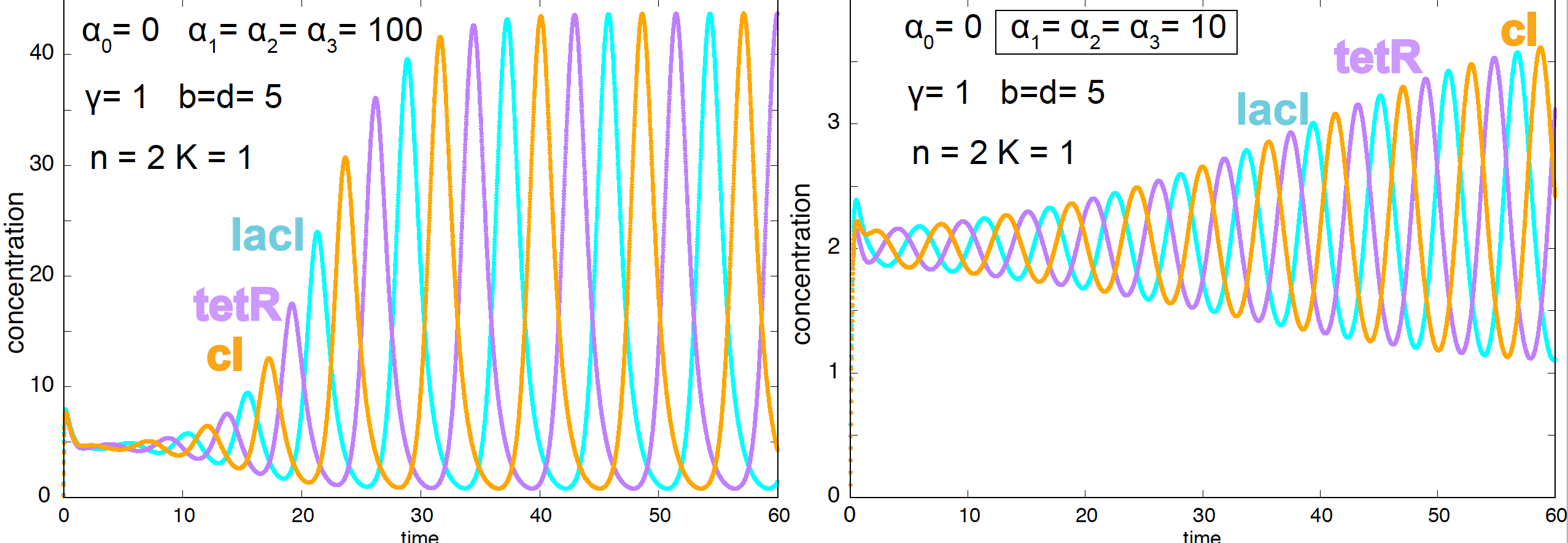
Figure 8. Oscillatory behavior of the E. coli repressilator.
The conditions under which the repressilator shows oscillations are
- High connectivity \(n >1\).
- \(\alpha_i\) parameters of similar magnitude.
- The effect of the constitutive promoter \(\alpha_0\) has to be small.
- The period of the oscillations is determined by the protein stability (the period increases as \(\delta\) decreases).
In Figure 9, we show a few examples testing the impact of changing different parameters in the oscillatory nature of the model.
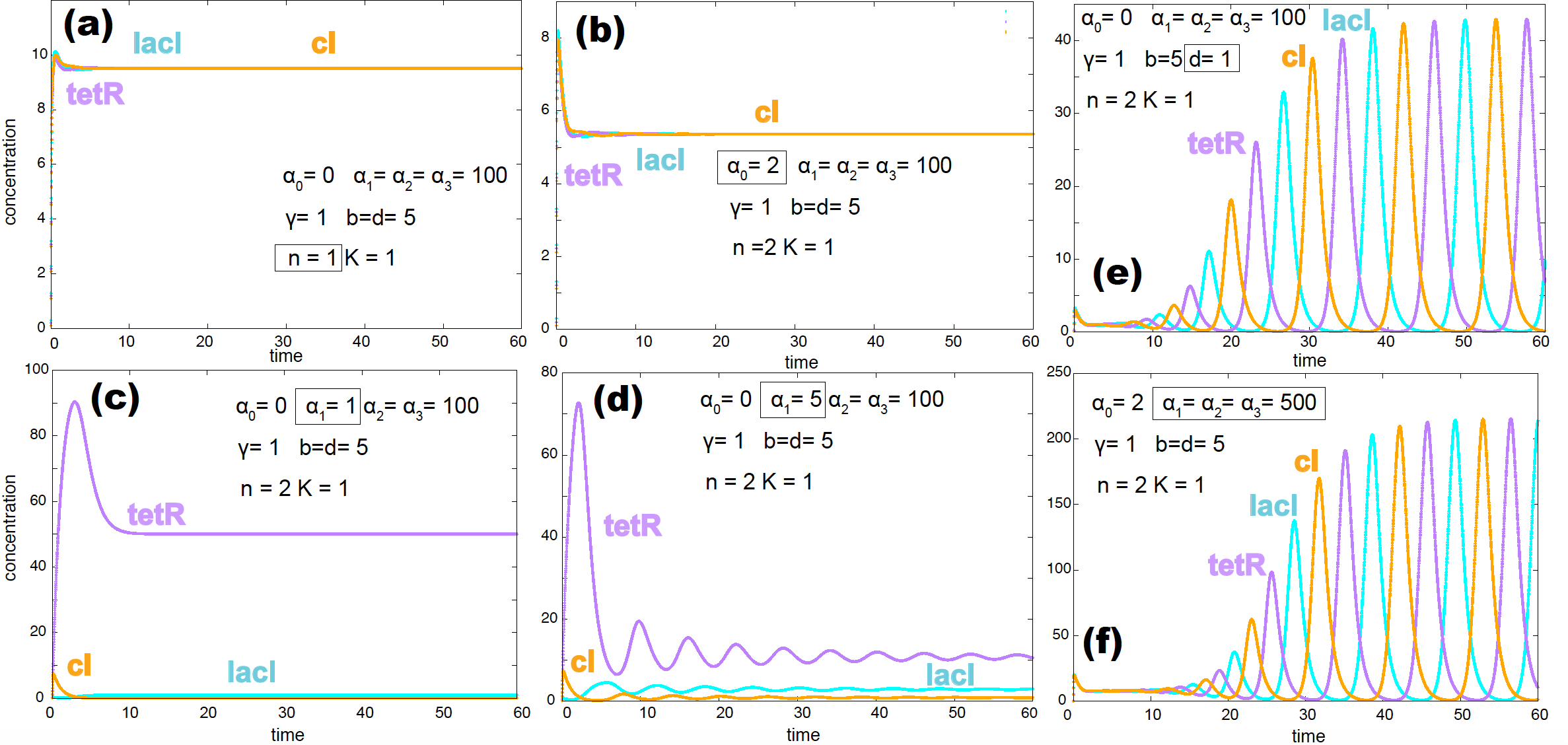
Figure 9. Several examples where the repressilator does not produce oscillations: (a) due to no cooperativity, (b) due to the effect of the non-inducible promoter, (c) & (d) due to a weak inducible promoter. Two examples that alter the period of the oscillations: (e) more stable proteins (small parameter d) increases the period of the oscillations. (f) Stronger inducible promoters increase the period of the oscillations as well. Altered parameters for each situation appear inside a box.
In their experimental implementation, Elowitz & Leibler found a lot of variability in the period and amplitude of the oscillations both as a function of time for one single cell and from cell to cell. Only about 40% of cells had oscillations.
In the homework, we will investigate another more stable and robust E. coli synthetic oscillator.
Stochastic simulations of the oscillations
The experimental implementation of the repressilator showed large variability in the oscillation both as a function of time (Figure 2 from paper), as well as from cell to cell (Figure 3 from paper). The authors wondered how much of that observed variability could be explained by the stochastic nature of the problem which is ignored by the deterministic solutions we have obtained so far.
As we studied in w10, we can implement the Gillespie algorithm to describe the stochastic behavior of the repressilator.
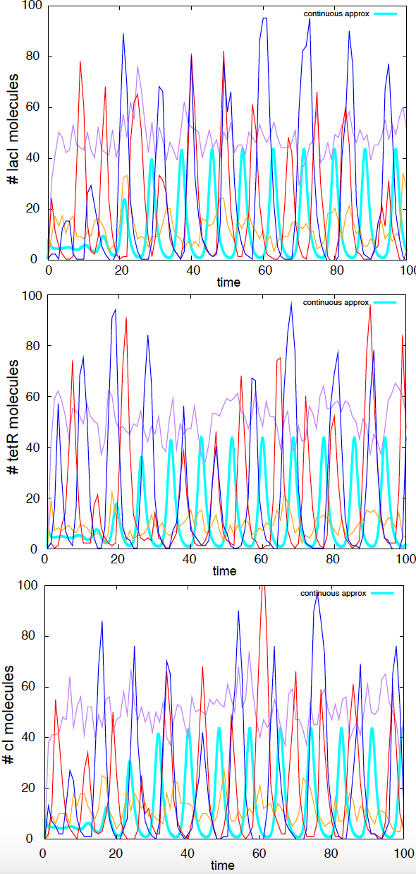
Figure 10. Stochastic simulations of the repressilator. Four independent stochastic simulations are depicted. Parameters are: a0 =0 a1=a2=a3=100, g=1,b=d=5,n=2. In Cyan, we depict the continuous solution.
The 15 reactions of the repressilator are
| r | reaction | propensity \(w_r\) | \(\eta\) |
|---|---|---|---|
| 1,2,3 | \(\emptyset \overset{\alpha_0}{\longrightarrow} m_i\) | \(\alpha_0\) | \(\eta(m_i)=+1\) |
| 4,5,6 | \(\emptyset \overset{\alpha_i}{\longrightarrow} m_i\) | \(\alpha_i \frac{1}{1+p_j^n}\) | \(\eta(m_i)=+1\) |
| 7,8,9 | \(m_i \overset{\gamma}{\longrightarrow} \emptyset\) | \(\gamma\ m_i\) | \(\eta(m_i)=-1\) |
| 10,11,12 | \(m_i \overset{\beta}{\longrightarrow} m_i + p_i\) | \(\beta\ m_i\) | \(\eta(p_i)=+1\) |
| 13,14,15 | \(p_i \overset{\delta}{\longrightarrow} \emptyset\) | \(\delta\ p_i\) | \(\eta(p_i)=-1\) |
where \(i=\{lacI, tetR, cI\}\) corresponds to \(j=\{CI, LacI, TetR\}\).
I have implemented the Gillespie algorithm for this stochastic process, using the same default parameters introduced above. The system does show large amount of variability in the shape and period of the oscillations for different stochastic simulations (see Figure 10).
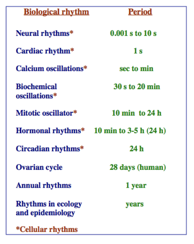
Figure 11. Time scale of different biological rhythms. Figure from 'Biomedical oscillations' by J. J. Tyson.
Molecular bases of a circadian rhythm in Drosophila
There are many oscillatory processes (rhythms) in living organisms (Figure 11). Amongst them are circadian rhythms that usually have a 24h period. Circadian rhythms are driven by the external cues of day and night on Earth, but they also can persist under constant illumination conditions. The molecular mechanisms behind circadian rhythms have been recently discovered by Michael Rosbash, Michael Young, Jeff Hall and others circa 1999.
As you can discover in this movie about the drosophila circadian rhythm, a large number of players are involved in the establishment of the drosophila circadian rhythm. There is one gene in particular, periodic (per), that is at the heart of the process. In this work, “A model for circadian oscillations in the Drosophila Period protein (PER)” by A. Goldbeter, a theoretical mechanism is established that supports the experimental observations about the per gene and PER protein.
The observations are
-
The concentration of the per RNA varies periodically.
-
The concentrations of the protein product PER also oscillates, but the oscillations follow those of the RNA by a few hours.
-
Only those cells in which PER is overproduced lose periodicity.
-
The protein product PER is multi-phosphorylated.
The model proposed is as follows (Figure 12)
-
PER (\(P_0\)) is produced in the cytoplasm from per RNA (\(R\)).
-
PER is phosphorylated several times while in the cytoplasm (\(P_1\), \(P_2\),…).
-
A \(2-\)phosphorylated form of cytoplasmatic PER (\(P_2\)) re-enters the nucleus (\(P_n\)).
-
Nuclear PER (\(P_n\)) interacts with the per promoter through a negative feedback loop, repressing the production of more per RNA.
-
The per RNA is very abundant, thus is not consumed in the production of PER.
-
Only the cytoplasmic phosphorylated form of the protein \(P_2\) is degraded.
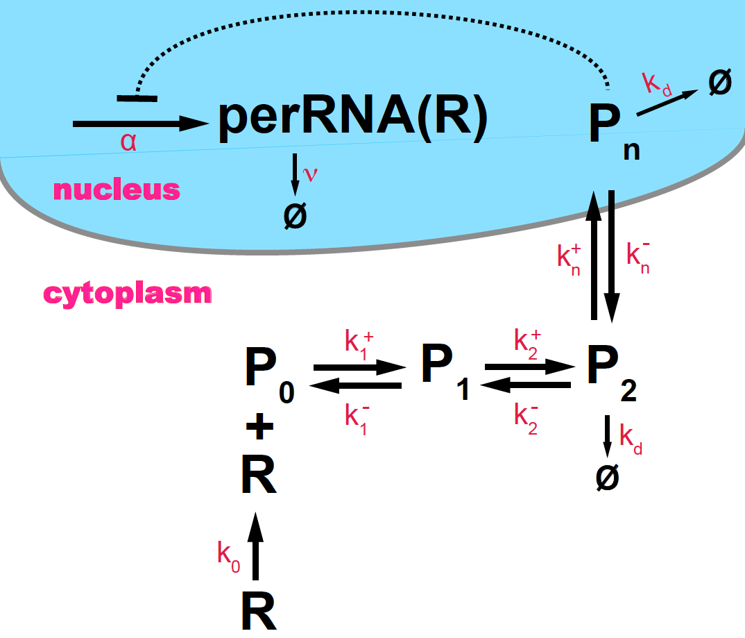
Figure 12. Scheme of circadian oscillations in PER protein (P) and per RNA (R), based on Goldbeter, 1995.
According to this mechanism, the simplest kinetic equations of the system are (assume \(N=2\))
\[\begin{aligned} \frac{d R}{d t} &= \alpha\ \frac{K^m}{K^m+{P_n}^m} - v\ R\\ \frac{d P_0}{d t} &= k_0 R - k_1^+ P_0 + k^-_1 P_1 \\ \frac{d P_1}{d t} &= k_1^+ P_0 - k_1^- P_1 + k^-_2 P_2 - k^+_2 P_1 \\ \frac{d P_2}{d t} &= k_2^+ P_1 - k_2^- P_2 + k_n^- P_n- k^+_n P_2 - k_d P_2 \\ \frac{d P_n}{d t} &= k^+_n P_2 - k_n^- P_n - k_d P_n\\ \end{aligned}\]where we have modeled the negative feedback loop by a Hill function of constant \(K\) and coefficient \(m\).
In Goldbeter’s work, the phosphorylation and de-phosphorilation reactions as well as the degradation of the per RNA and the PER protein are proposed to be enzymatic reactions, thus instead of the simple (exponentially decaying) form that I introduced above, they are assumed to follow the Michaelis-Menten enzymatic behavior. Let’s us take a short detour to look at the kinetics of enzymatic reactions under Michaelis-Menten conditions.
In Goldbeter’s work, only the phosphorylated \(P_2\) form of PER, but not the nuclear form \(P_n\), can decay. In this implementation, we generalize so that both forms of the PER can decay enzymatically with the same rate constants.
Michaelis-Menten kinetics
The phosphorylation/de-phosphorylation reactions do not occur in isolation, but are mediated by an enzyme, and usually requires the formation of an intermediate compound \(C\) (Figure 13)
\[P_0 + E \underset{k^-}{\overset{k^+}{\rightleftharpoons}} C \overset{\alpha}{\longrightarrow} P_1 + E.\]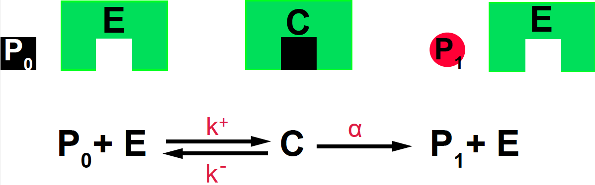
Figure 13. Michaelis-Menten mechanism for an enzyme-mediated reaction.
The kinetic equations are given by
\[\begin{aligned} \frac{d C}{d t} &= k^+ P_0\ E - k^- C - \alpha C.\\ \frac{d P_1}{d t} &= \alpha\ C \end{aligned}\]We are going to assume that the reversible reaction that forms the complex \(C\) is much faster than the dissociation into the new species \(P_1\),
that is
\[k^+,k^- >> \alpha\]in that case, we expect that the concentration of \(C\) reaches steady state much faster than that of \(P_1\),
\[\begin{aligned} \frac{d C}{d t} &\approx k^+ P_0\ E - k^- C.\\ \end{aligned}\]Because the total concentration of the enzyme \(E_T\) is the sum of the concentration of being bound and unbound, we have \(E_T = E+C\), so at steady state
\[k^+ P_0\ (E_T - C) - k^- C = 0\]or
\[C = E_T\ \frac{P_0}{\frac{k^-}{k^+} + P_0}\]then the kinetic equation for the product \(P_1\) is a function of the substrate \(P_0\) given by
\[\frac{d P_1}{d t} = \alpha\ E_T\ \frac{P_0}{K_M + P_0}\]where the Michaelis-Menten constant is given by
\[K_M = \frac{k^-}{k^+}.\]Circadian oscillations
The Drosophila per/PER kinetic equations introducing the Michaelis-Menten enzymatic nature of four phosphorylation/de-phosphorylation reactions (with Michaelis-Menten constants \(K1,K2,K3, K4\)) and the two per RNA and PER decays (characterized by Michaelis-Menten constants \(Km\) and \(Kd\) respectively) are
\[\begin{aligned} \frac{d R}{d t} &= \alpha\ \frac{K^m}{K^m+{P_n}^m} - v\ \frac{R}{Km+R}\\ \frac{d P_0}{d t} &= k_0\ R - k_1^+ \frac{P_0}{K1+P_0} + k^-_1 \frac{P_1}{K2+P_1} \\ \frac{d P_1}{d t} &= k_1^+ \frac{P_0}{K1+P_0} - k_1^- \frac{P_1}{K2+P_1} - k^+_2 \frac{P_1}{K3+P_1} + k^-_2 \frac{P_2}{K4+P_2} \\ \frac{d P_2}{d t} &= k_2^+ \frac{P_1}{K3+P_1} - k_2^- \frac{P_2}{K4+P_2} + k_n^- P_n- k^+_n P_2 - k_d \frac{P_2}{Kd+P_2} \\ \frac{d P_n}{d t} &= k^+_n P_2 - k_n^- P_n - k_d \frac{P_n}{Kd+P_n}\\ \end{aligned}\]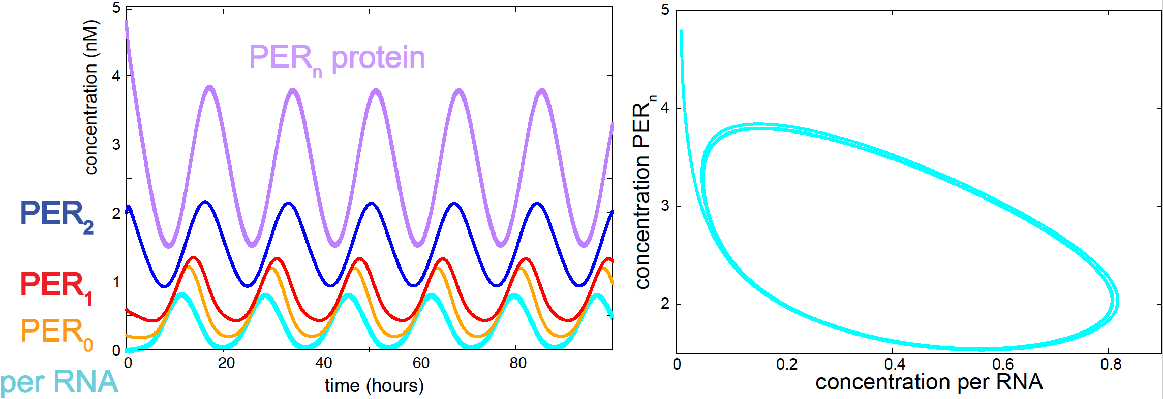
Figure 14. Oscillations of per RNA and PER protein according to the Goldbeter model.
The values of the parameters are not known in principle. They are mostly set by hand, by trial and error by requesting that the system has some of the observed features of the oscillator:
- Oscillations have a period of approximately 24 hours.
- The peak of the protein occurs a few hours before the peak of the RNA.
The set of parameters below does produce large and stable oscillations both for the per RNA and the PER protein (see Figure 14).
| parameter | Description | value |
|---|---|---|
| \(\alpha\) | per RNA production | 0.5 nM/h |
| \(v\) | per RNA degradation | 0.3 nM/h |
| \(m\) | cooperativity coefficient of PER binding | 4 |
| \(K\) | Hill constant | 2 nM |
| \(k_0\) | translation rate | 2 nM/h |
| \(k_1^+ = k_2^+\) | PER phosphorylation rate | 6 nM/h |
| \(k_1^- = k_2^-\) | PER de-phosphorylation rate | 3 nM/h |
| \(k_n^+\) | PER nuclear import rate | 2 nM/h |
| \(k_n^-\) | PER nuclear export rate | 1 nM/h |
| \(k_d\) | PER degradation rate | 0.4 nM/h |
| \(Km\) | Michaelis constant for RNA degradation | 0.2 nM |
| \(Kd\) | Michaelis constant for PER degradation | 0.1 nM |
| \(K1=K3\) | Michaelis constant for PER phosphorylation | 1.5 nM |
| \(K2=K4\) | Michaelis constant for PER de-phosphorylation | 2.0 nM |
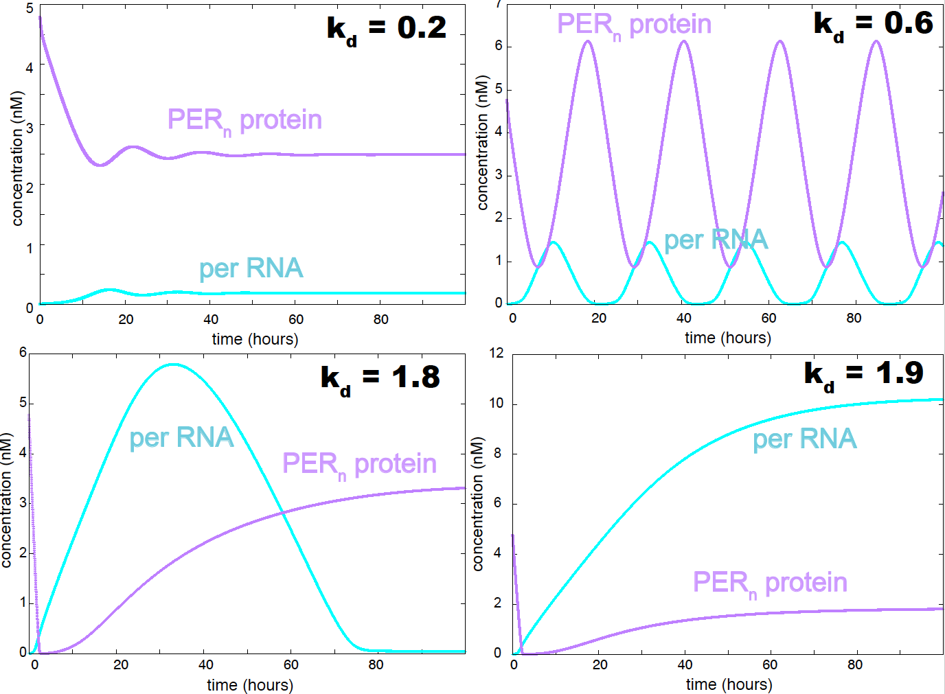
Figure 15. Behavior of the goldbeter model as a function of the PER decay constant. In this version of the model both P2 and Pn are allowed to decay enzymatically.
The oscillations in Figure 14 are robust and stable. An important parameter controlling the nature of the oscillations is the PER decay constant \(k_d\). Small values of \(k_d\) results in a weakly oscillating system with dampened oscillations. The oscillations become stronger as \(k_d\) increases, passed some value of \(k_d\) the system becomes non-oscillatory (see Figure 15). If only the \(P_2\) form of the PER protein is allowed to degrade (as in the original Goldbeter model), oscillations are favored, and the range of values of \(k_d\) that result in an oscillatory behavior is larger.
As we saw in the video, there are many more players in the system. PER forms a complex with protein timeless (TIM). The transcription of TIM is co-regulated with that of PER, and the light dependence of the oscillatory cycle results from the fact that TIM is degraded by light. Theoretical models describing the interactions between PER and TIM have been constructed, see for instance “A model for the circadian rhythm in Drosophila incorporating the formation of a complex between the PER and TIM proteins” by Leloup & Goldbeter, 1999.