MCB111: Mathematics in Biology (Fall 2024)
- stochastic gating of a single ion channel
- Fluctuating populations of RNAs in a cell: a Birth-Death process
- Gene regulation
week 10:
Molecular Dynamics as a Markov Process
For these lectures, I have followed Chapter 8 of Philip Nelson’s book “Physical models of living systems”. I have also followed the more comprehensive, but really great review “Stochastic simulations, applications to biomolecular networks” by Gonze and Ouattara, 2014. A beautiful description of Ion channel gating as a Markov process is given by G. D. Smith in “Modeling of Stochastic Gating of Ion Channels”.
stochastic gating of a single ion channel
Cells contain numerous ion channels. Ion channels are transmembrane proteins that strand the cell membrane and facilitate (by opening and closing) the movement of many different molecules in-and-out of the cell.
Using patch clamp techniques, we can measure the dynamics of a single ion channel. Using a continuous-time Markov process with two states (open and close), we can model the stochastic gating of a single ion channel.
A two-state continuous-time Markov process
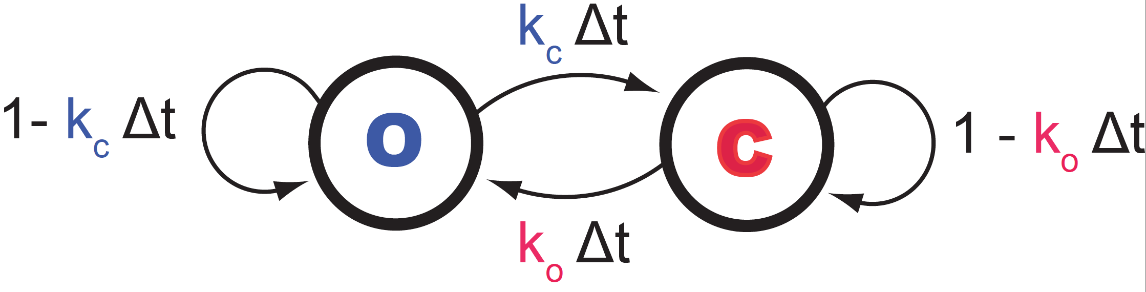
Figure 1. The two-state ion channel continuous time Markov model. Kc is the instantaneous probability of the channel to close, and Ko is the instantaneous probability of the channel opening.
The dynamics of the ion channel gating can be described as
\[O(open) \overset{k_c}{\underset{k_o}{\rightleftharpoons}} C(close)\]where \(k_o\) and \(k_c\) are the reaction constants of the process.
These reaction constants can be interpreted as probabilities per unit time of the stochastic process of the channel opening and closing. That is
-
The probability of the channel transitioned from C to O between time \(t\) and \(t+\Delta t\) is given by
\[t(C\rightarrow O) \equiv P(O, t+\Delta t\mid C,t) = k_o \Delta t.\] -
The probability of the channel transitioned from O to C between time \(t\) and \(t+\Delta t\) is given by
\[t(O\rightarrow C) \equiv P(C, t+\Delta t\mid O,t) = k_c \Delta t.\] -
Thus, the probabilities that the channel remained closed (open) from \(t\) to \(t+\Delta t\) are given by
\[\begin{aligned} t(C\rightarrow C) \equiv P(C, t+\Delta t\mid C,t) &= 1 -k_o \Delta t\\ t(O\rightarrow O) \equiv P(O, t+\Delta t\mid O,t) &= 1 -k_c \Delta t. \end{aligned}\]
This is a Markov process, in which the state \(S_i=\{O,C\}\), at a given time \(i\Delta t\) is determined by the previous state \(S_{i-1}\).
\[S_0 \underset{t(S_0\rightarrow S_1)}{\overset{\Delta t}{\longrightarrow}} S_1 \underset{t(S_1\rightarrow S_2)}{\overset{\Delta t}{\longrightarrow}} S_2 \underset{t(S_2\rightarrow S_3)}{\overset{\Delta t}{\longrightarrow}} \ldots \underset{t(S_{N-1}\rightarrow S_N)}{\overset{\Delta t}{\longrightarrow}} S_N\]We can represent this continuous-time stochastic process as a two state Markov process, see Figure 1. Notice how the two probabilities that emerge from a given state (either O or C) sum up to one.
The transition probability matrix
Introducing
\[\begin{aligned} P(O\mid t)&\quad \mbox{ probability of being open at time}\ t\\ P(C\mid t)&\quad \mbox{ probability of being closed at time}\ t \end{aligned}\]such that
\[P(O\mid t) + P(C\mid t) = 1 \quad \mbox{ for all}\ t's.\]One can write, using the graphical representation described in Figure 1,
\[\begin{aligned} P(O\mid t+\Delta t)&= \left. \begin{array}{rl} + k_o \Delta t & P(C\mid t)\\ + (1-k_c \Delta t) & P(O\mid t) \end{array} \right. \\ P(C\mid t+\Delta t)&= \left. \begin{array}{rl} + k_c \Delta t & P(O\mid t)\\ + (1-k_o \Delta t) & P(C\mid t) \end{array} \right. \end{aligned}\]The above equations can be re-written as
\[{P(O\mid t+\Delta t) \choose P(C\mid t+\Delta t)} = \left( \begin{array}{cc} 1-k_c \Delta t & k_o \Delta t \\ k_c \Delta t & 1-k_o \Delta t & \end{array} \right) {P(O\mid t) \choose P(C\mid t)}\]Introducing the transition matrix \(T\) given by
\[T = \left( \begin{array}{cc} t(O\rightarrow O) & t(C\rightarrow O) \\ t(O\rightarrow C) & t(C\rightarrow C) & \end{array} \right) = \left( \begin{array}{cc} 1-k_c \Delta t & k_o \Delta t \\ k_c \Delta t & 1-k_o \Delta t & \end{array} \right),\]we can write
\[{P(O\mid t+\Delta t) \choose P(C\mid t+\Delta t)} = T\ {P(O\mid t) \choose P(C\mid t)}.\]The matrix \(T\) is such that the sum of the probabilities in each column is 1.
Using vector notation
\[\vec{P}(t) = {P(O\mid t) \choose P(C\mid t)},\]we can write
\[\vec{P}(t+\Delta t) = T\ \vec{P}(t).\]Then, for \(t +2\Delta t\), we have
\[\vec{P}(t+2\Delta t) = T\ \vec{P}(t+\Delta t) = T^2\ \vec{P}(t),\]and in general for \(t + n\Delta t\), we have
\[\vec{P}(t+n\Delta t) = T^n\ \vec{P}(t).\]This equation is usually referred as the Chapman-Kolmologov equation. This is a general result for all continuous-time Markov processes.
Deterministic solution
The state equations can be re-written as
\[\begin{aligned} P(C\mid t+\Delta t) - P(C\mid t) &= k_c\Delta t\ P(O\mid t) - k_o\Delta t P(C\mid t)\\ P(O\mid t+\Delta t) - P(O\mid t) &= k_o\Delta t\ P(C\mid t) - k_c\Delta t P(O\mid t). \end{aligned}\]that is
\[\begin{aligned} \frac{P(C\mid t+\Delta t) - P(C\mid t)}{\Delta t} &= k_c\ P(O\mid t) - k_o\ P(C\mid t)\\ \frac{P(O\mid t+\Delta t) - P(O\mid t)}{\Delta t} &= k_o\ P(C\mid t) - k_c\ P(O\mid t). \end{aligned}\]If we take the limit of very small time intervals \(\Delta t \rightarrow 0\), then the transition equations can be written in continuous form as
\[\begin{aligned} \frac{d P(O\mid t)}{d t} &= k_o\ P(C\mid t) - k_c\ P(O\mid t)\\ \frac{d P(C\mid t)}{d t} &= k_c\ P(O\mid t) - k_o\ P(C\mid t). \end{aligned}\]Using the relationship \(P(C\mid t) = 1 - P(O\mid t)\), we have
\[\begin{aligned} \frac{d P(O\mid t)}{d t} &= k_o - (k_c+k_o)\ P(O\mid t)\\ \frac{d P(O\mid t)}{d t} &= k_c - (k_c+k_o)\ P(C\mid t) \end{aligned}\]The time-dependent solutions are given by
\[\begin{aligned} P(O\mid t) &= \frac{k_o}{k_c+k_o} + \left(P(O\mid 0) - \frac{k_o}{k_c+k_o}\right)e^{-(k_c+k_o)t}\\ P(C\mid t) &= \frac{k_c}{k_c+k_o} + \left(P(C\mid 0) - \frac{k_c}{k_c+k_o}\right)e^{-(k_c+k_o)t}. \end{aligned}\]Using the Chapman-Kolmologov equation in continuous form
\[\vec{P}(t+\Delta t) - \vec{P}(t) = (T - I)\ \vec{P}(t).\]Let’s introduce the matrix \(Q\)
\[Q = \frac{1}{\Delta t}\ \left(T-I\right) = \left( \begin{array}{cc} -k_c&k_o\\ k_c&-k_o \end{array} \right).\]The matrix \(Q\) represents the changes per unit time from and to a given state. Because the sum of all changes have to be zero. We observe that as the sum of each column in \(Q\) is zero.
Then, we have in the limit \(\Delta t \rightarrow 0\),
\[\frac{d\vec{P}(t)}{dt} = Q\ \vec{P}(t).\]The general solution for this equation is
\[\vec{P}(t) = \vec{P}(t=0)\ e^{t\ Q}.\]This is a general result for all continuous-time Markov processes.
For the particular Ion channel case, we have found already the solutions to the general equation given by
\[\begin{aligned} P(O\mid t) &= \frac{k_o}{k_c+k_o} + \left(P(O\mid 0) - \frac{k_o}{k_c+k_o}\right)e^{-(k_c+k_o)t}\\ P(C\mid t) &= \frac{k_c}{k_c+k_o} + \left(P(C\mid 0) - \frac{k_c}{k_c+k_o}\right)e^{-(k_c+k_o)t}. \end{aligned}\]In general, in a cell there are many channels working together, if we consider the average of many of such ion channels, we find that the average state at a given time \(t\) is
\[\begin{aligned} \langle channel(t)\rangle &= 1\times P(O\mid t) + 0\times P(C\mid t)\\ &= P(O\mid t)\\ &= \frac{k_o}{k_c+k_o} + \left(P(O\mid 0) - \frac{k_o}{k_c+k_o}\right)e^{-(k_c+k_o)t} . \end{aligned}\]In Figure 2, we show both this continuous average (in blue), as well as the sample average of 100 different stochastic simulations (in purple). This is the code used to produce Figure 2.
The steady-state solution
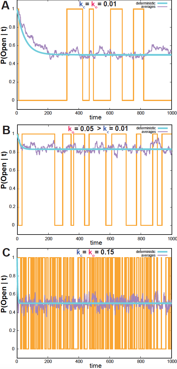
Figure 2. Single ion channel simulations. In yellow, the result of one simulation using the Monte Carlo algorithm. In purple, the average of 100 such simulations. In blue, the continuous time solution. (A) Ko=Kc = 0.01, (B) Ko=0.05, Kc = 0.01, (C) Ko=Kc=0.15. We assume the channel is open at t=0.
In the limit of large time \(t\), we obtain the steady state probabilities which are given by
\[\begin{aligned} P(O\mid \infty) &= \frac{k_o}{k_c+k_o}\\ P(C\mid \infty) &= \frac{k_c}{k_c+k_o}. \end{aligned}\]It is called steady-state, because in this limit the probabilities of staying open/close do not depend on time anymore
\[\frac{P(O\mid t)}{dt} = 0\quad \mbox{at steady state}.\]An alternative form of finding the steady-state solution, is by finding the solution to the differential equations for which
\[\frac{P(O\mid t)}{dt} = 0.\]In Figure 2, we see how the steady state (in blue) behaves as a function of the rates.
-
If \(k_o=k_c\) (Figure 2A), then
\[P(O\mid \infty) = P(C\mid \infty) = \frac{1}{2}.\] -
As the rates become larger (Figure 2C), the system reaches steady state (blue line) faster.
Dwell Times
We can calculate the expected time that the channel will remain open (or closed).
If we assume the channel is O at time \(t\), the probability that it stays open until \(t+\tau\), assuming \(m\) infinitesimal steps, such that \(\tau = m\ \Delta t\)
\[\begin{aligned} P(O, t+\tau\mid O,t) &= P(O, t+\tau\mid O,t+\tau-\Delta t)\\ &\times P(O, t+\tau-\Delta t\mid O,t+\tau-2\Delta t)\\ &\times \ldots\\ &\times P(O, t+\Delta t\mid O,t)\\ &= \left(1-k_c\Delta t\right)^m\\ &= \left(1-k_c\ \frac{\tau}{m}\right)^m. \end{aligned}\]In the limit of \(\Delta t\rightarrow 0\) and \(m\rightarrow \infty\) such that \(\tau = m\Delta t\) remains constant, we have
\[\begin{aligned} P(O, t+\tau\mid O,t) &= \lim_{m\rightarrow \infty} \left(1-k_c\ \frac{\tau}{m}\right)^m\\ &= e^{-k_c\ \tau} \end{aligned}\]Finally, the probability of a dwell time \(\tau\) requires adding the normalization term \(k_c\) which is the contribution of changing to close after \(t+\tau\), then
\[P_O(\tau) = k_c\ e^{-k_c\ \tau}.\]and the expectation is
\[\langle \tau \rangle_O = \int_0^1 \tau\ k_c\ e^{-k_c\ \tau} d\tau = \frac{1}{k_c}.\]Similarly for the dwell time in the closed state, resulting in
\[\langle \tau\rangle_O = \frac{1}{k_c}\\ \langle \tau\rangle_C = \frac{1}{k_o}.\]In Figure 2, one can see this behavior. For small rates, the dwell times are large, and the channels stays in one state for a while (Figure 2A, where the expected dwell time is 100 time units for both states). When the rates become smaller, the dwell times are small and the channels rapidly fluctuates between the open and closed state (Figure 2C. where the expected dwell time is 1 time unit for both states).
Stochastic simulations: Monte Carlo algorithm
When the fluctuation times are not very small, the opening/closing of an ion channel is not deterministic but stochastic. The transition matrix
\[T = \left( \begin{array}{cc} 1-k_c \Delta t & k_o \Delta t \\ k_c \Delta t & 1-k_o \Delta t & \end{array} \right)\]is such that \(T_{ij}\) gives us the probability of transitioning from one state (O or C) at time \(t\), to the state (O or C) at time \(t+\Delta t\).
We can simulate this process computationally.
Draw a random number \(x\) between 0 an 1,
-
If the current state is O,
- if \(x < k_c\Delta t\), then the channel closes,
- otherwise it stays O
-
If the current state is C,
- if \(x < k_o\Delta t\), then the channel opens,
- otherwise it stays C.
In Figure 2, I show simulations of the ion channel system, for different values of \(k_c\) and \(k_o\). Figures 2A and 2B show the difference in steady-state between the case \(k_c=k_c\) and \(k_o>k_c\). Figure 2C shows how as \(k_c\) and \(k_o\) increase in magnitude, the dwell time in each state becomes smaller, and the system switches between open and close states much faster than before
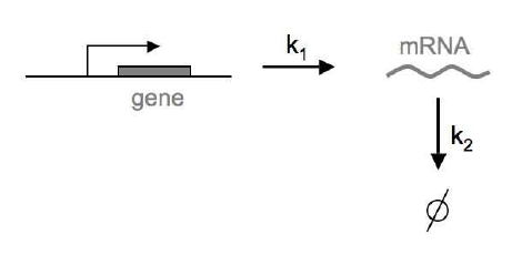
Figure 3. RNA synthesis/degradation as a birth-death process. k1 is the rate (probability per unit time) of RNA synthesis, and k2 is the rate of RNA degradation. We assume that these rates are constant. Figure from Gonze and Ouattara, 2014.
Fluctuating populations of RNAs in a cell: a Birth-Death process
The production and degradation of RNA molecules in a cell is another process that has been successfully model as a continuous-time Markov process. We assume there is rate (probability per unit time) \(k_1\) of an RNA molecule being produced, and another rate \(k_2\) for the RNA molecule to be degraded. We can write the process as a set of two reactions:
\[\begin{aligned} \emptyset &\overset{k_1}{\longrightarrow} RNA \quad \mbox{RNA synthesis (birth)}\\ RNA &\overset{k_2}{\longrightarrow} \emptyset \quad \quad\, \mbox{RNA degradation (death)} \end{aligned}\]In our simple model, we are going to assume that these rates are constant in time, but they could easily be time-dependent.
There is a whole machinery of protein-RNA molecules behind both transcription and RNA degradation, which we are ignoring here. We are just representing the combined output of those two processes, that is, the number of molecules of a given RNA as a function of time.
The birth-death master equation
The process of RNA synthesis/degradation is fundamentally stochastic. We introduce the probability
\[P(R\mid t)\]defined as the probability of having \(R\) RNA molecules at time \(t\). Knowing this probability distribution would give us information about the state of the system at all times.
We are going to assume that in a very small time interval \(\Delta t\), only one of the two possible reactions, or none at all is going to occur. (Double event would occur with probability proportional to \((\Delta t)^2\) which we assume is very very small.)
We can write what the probability distribution will be at time \(t+\Delta t\), \(P(R\mid t+\Delta t)\), as a function of the probability distribution at time \(t\), \(P(R\mid t)\), after considering all possible single-reaction events that can occur in the interval \(\Delta t\).
In general terms, if we have \(R\) reactions (two for our RNA processing question)
\[\begin{aligned} P(X\mid t+\Delta t) = &\sum_{r=1}^R P(X-\eta_r\mid t)\ P(\mbox{change in}\ \Delta t\ \mbox{due to r})\\ &+ P(X\mid t)\ P(\mbox{no change in}\ \Delta t), \end{aligned}\]where \(X=(X_1,\ldots,X_n)\) is the total number of molecules of all species \(n\) in the system. For each reaction \(r\) and each species \(X_i\), \(\eta_r^i\) is the difference between the coefficient in the right and left sides of the reaction of species \(X_i\) in reaction \(r\). For instance, \(\eta_b(R) = 1\) for the RNA synthesis (birth) reaction, and \(\eta_d(R) = -1\) for the RNA degradation (death) reaction.
As for the probabilities of the possible individual events that can occur in \(\Delta t\), we have
\[P(\mbox{change in}\ \Delta t\ \mbox{due to r}) = w_r(X-\eta_r) \Delta t\] \[P(\mbox{no change in}\ \Delta t) = 1 - \sum_r w_r(X)\Delta t\]where \(w_r(X_1,\ldots,X_n)\) is called the “propensity” of the reaction, and it is defined as the probability that the reaction will occur per unit time.
In summary, for \(R\) reactions, with reactivities \(w_r(X)\), and coefficients \(\eta_r\) for \(1\leq r\leq R\), the recursion equation is given by
\[\begin{aligned} P(X\mid t+\Delta t) = &\sum_{r=1}^R P(X-\eta_r\mid t)\ w_r(X-\eta_r) \Delta t\\ &+ P(X\mid t)\ \left(1 - \sum_r w_r(X)\Delta t\right), \end{aligned}\]In our case, there is only one species, and two reactions
- X = R, the number of RNA molecules
-
For the birth reaction \(\emptyset \overset{k_1}{\longrightarrow} RNA\)
\[\eta_b = 1\] \[w_b(R) = k_1\] -
For the death reaction, \(RNA \overset{k_2}{\longrightarrow} \emptyset\)
\[\eta_d = -1\] \[w_d(R) = k_2 R\]since any of the existing \(R\) molecules could be the one to be degraded.
Explicitly, we have
\[\begin{aligned} P(R\mid t+\Delta t) &=\\ &\begin{array}{rl} + k_1\ \Delta t\ P(R-1\mid t) & \mbox{change at}\ \Delta t\ \mbox{do to RNA synthesis reaction}\\ + k_2\ (R+1)\ \Delta t\ P(R+1\mid t) & \mbox{change at}\ \Delta t\ \mbox{do to RNA degradation reaction}\\ + (1-k_1\Delta t -k_2 R\Delta t)\ P(R\mid t) & \mbox{no change over}\ \Delta t. \end{array} \end{aligned}\]This is known as the master equation.
The process is Markovian as the number of RNA molecules at a given time depends only on the previous state, but not on its history.
The master equation can be re-written a
\[\begin{aligned} \frac{P(R\mid t+\Delta t) - P(R\mid t)}{\Delta t} &= + k_1\ P(R-1\mid t) + k_2\ (R+1)\ P(R+1\mid t) -(k_1 +k_2 R)\ P(R\mid t). \end{aligned}\]And in the limit of \(\Delta t\) very small,
\[\begin{aligned} \frac{d P(R\mid t)}{d t} &= + k_1\ P(R-1\mid t) + k_2\ (R+1)\ P(R+1\mid t) -(k_1 +k_2 R)\ P(R\mid t). \end{aligned}\]If all the rates are constant, this equation can be solved analytically. You can find the solution and how to get it in this paper for instance. Here we are going to concentrate on
- Finding the deterministic solution in the limit of very large number of particles.
- Finding stochastic solutions by simulation using the Gillespie algorithm.
The deterministic approach (huge numbers of particles)
Some RNAs are very abundant in a cell. When \(R\) is very large, changing it by one molecule is insignificant. In that case, it makes more sense to look at the dynamics of the averages the master equation above.
Multiplying by \(R\) and summing to all possible values of \(R\) in both sides of the master equation above, we have
\[\begin{aligned} \sum_R R\ \frac{d P(R\mid t)}{d t} &= + k_1\ \left[ \sum_R R\ P(R-1\mid t) - \sum_R R \ P(R\mid t)\right] + k_2\ \left[ \sum_R R\ (R+1)\ P(R+1\mid t) - \sum_R R^2\ P(R\mid t)\right]. \end{aligned}\]A change of variable in the first and third right-hand side terms results in,
\[\begin{aligned} \sum_R R\ \frac{d P(R\mid t)}{d t} &= + k_1\ \left[ \sum_R (R+1)\ P(R\mid t) - \sum_R R\ P(R\mid t)\right] + k_2\ \left[ \sum_R (R-1)R\ P(R\mid t) - \sum_R R^2\ P(R\mid t)\right]. \end{aligned}\]Which can be simplified to
\[\begin{aligned} \frac{d \sum_R R\ P(R\mid t)}{d t} &= + k_1\ \sum_R P(R\mid t) - k_2\ \sum_R R\ P(R\mid t). \end{aligned}\]or
\[\frac{d \langle R\rangle_t}{d t} = k_1 - k_2 \langle R\rangle_t.\]The solution of this differential equation is
\[\langle R\rangle_t = \langle R\rangle_0\ e^{-k_2 t} + \frac{k_1}{k_2}\left(1-e^{-k_2 t}\right),\]where \(\langle R\rangle_0\) is the average number of RNA molecules at time \(t=0\).
The steady-state
If we assume that \(\langle R\rangle_0 = 0\), then
\[\langle R\rangle_t = \frac{k_1}{k_2}\left(1-e^{-k_2 t}\right),\]which has the steady state solution
\[\langle R\rangle_\infty = \frac{k_1}{k_2}.\]Stochastic simulation: The Gillespie algorithm
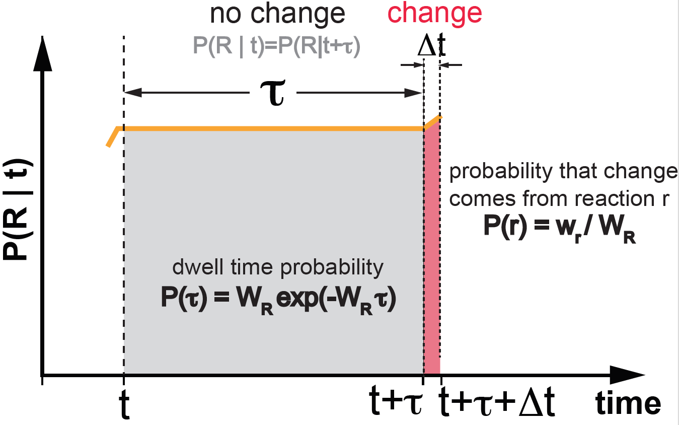
Figure 4. The Gillespie algorithm. wr is the propensity of a given reaction r. The sum of all propensities is given by WR.
Having the large-number deterministic solution is useful, but RNA synthesis and degradation is mostly stochastic.
Let’s go back to the master equation. If the rates \(k_1\) and \(k_2\) are constants, there is an analytical solution. However, oftentimes a simulation is more productive than trying to find analytical solutions.
We could use a brute force Monte Carlo simulation as the one we described above for the ion channel gating. There is a different and much faster and exact algorithm that we can use here, the Gillespie algorithm.
In the Monte Carlo algorithm I used in Figure 1 for ion channel gating, I sampled at all possible time increments \(\Delta t\). The Gillespie algorithm avoids taking a sample at every single time increment by estimating the dwell time in which no change is going to occur.
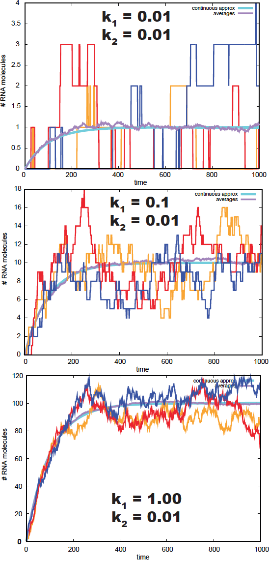
Figure 5. Gillespie simulation of 3 time series of an RNA population. In blue, we depict the deterministic solution. In purple, we depict the averages over 200 simulations.
The Gillespie algorithm takes advantage of dwell times, and jumps from one dwell time to the next avoiding sampling in at all intermediate times. The Gillespie algorithm consists of two steps, and it works as follows (see Figure 4)
-
(1) Sample a dwell time \(\tau\)
The time \(\tau\) until a reaction occurs with probability
\[P(\tau) = W_R e^{-W_R \tau},\]where \(W_R = \sum_r w_r\) is the sum of the propensities of all reactions.
This dwell time probability can be calculated similarly to how we did it for the dwell times of a gated ion channel. The probability of dwell time \(\tau\) is given by the probability that the species in the reaction \(X=\{X_1,\ldots, X_N\}\) remain unchanged from time \(t\) to \(t+\tau\), multiplied by the probability that there is a change immediately after at time \(t+\tau+\Delta t\). That is,
\[\begin{aligned} P(\tau) \propto\, & \,P(X, t+\tau\mid X,t) \\ \propto\, & \,P(X, t+\tau\mid X,t) \\ \propto\, & \,P(X, t+\tau\mid X,t+\tau-\Delta t) \\ \, & \,\times \,P(X, t+\tau-\Delta t\mid X,t+\tau-2\Delta t) \\ \, & \,\times \ldots\\ \, & \,\times \,P(X, t+\Delta t\mid X,t)\\ \propto\, & \,\left(1- \sum_r w_r(X)\Delta t\right)^m\\ \propto\, & \.\,\left(1-W_R\ \frac{\tau}{m}\right)^m. \end{aligned}\]In the limit of \(\Delta t\rightarrow 0\) and \(m\rightarrow \infty\) such that \(\tau = m\Delta t\) remains constant, we have
\[P(\tau) \propto \lim_{m\rightarrow \infty} \left(1-W_R\ \frac{\tau}{m}\right)^m = e^{-W_R\ \tau}.\]Adding the normalization constant \(W_R\) (the instantaneous total probability of change), we obtain for the probability of dwell times \(\tau\) as,
\[P(\tau) = W_R\, e^{-W_R\ \tau}.\] -
(2) Sample a reaction to take place in \(\Delta t\).
Of all possible reactions that could occur in \(\Delta t\), we sample them according to their propensity \(w_r\), that is,
\[P(r) = w_r / W_R.\]
The Gillespie algorithm samples exactly the stochastic process described by the master equation.
For the particular birth-death model of RNA synthesis/degradation, described by the reactions
| r | reaction | propensity | \(\eta(R)\) |
|---|---|---|---|
| 1 | \(\emptyset \overset{k_1}{\longrightarrow} RNA\) | \(k_1\) | \(+1\) |
| 2 | \(RNA \overset{k_2}{\longrightarrow} \emptyset\) | \(k_2 R\) | \(-1\) |
the Gillespie algorithm works as follows,
-
We keep a count of the current number of RNA molecules \(R\) at time \(t\),
-
sample a dwell time \(\tau\) from the exponential distribution
\[P(\tau) = W_R e^{-W_R \tau},\]where \(W_R = k_1+k_2 R\).
Then \(t\) increases to \(t+\tau\)
-
We draw a random number \(0<x\leq 1\) such that
- If \(x < \frac{k_1}{k_1+k_2 R}\), then \(R\) increases by one molecule, \(R \rightarrow R+1\)
- otherwise, \(R\) decreases by one molecule, \(R \rightarrow R-1\)
- Update the number of RNA molecules
- Go back to sampling another dwell time until we decide to end the reaction.
I have simulated several stochastic processes using the Gillespie algorithm, given in Figure 5. We observe how the averages converge to the limit \(k_1/k_2\). We also observe that as the number of RNA molecules increases, the simulations w approach the deterministic solution.
Gene regulation
This approach to modeling the expression and regulation of a single gene is derived from this work: “Intrinsic noise in gene regulation” by Thattai and Oudenaarden, PNAS 2001; and “Regulation of noise in the expression of a single gene” by Ozbudak et al., Nature 2002.
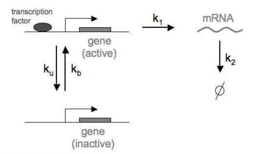
Figure 6. Transcriptional bursting as a birth-death process. Genes spontaneously transition from active to inactive with fixed probabilities per unit time: ku (from active to inactive) and kb (from inactive to active).
Transcriptional bursting
Here we consider the same RNA processing question but where we also model the activation and deactivation of the gene responsible from producing the RNA. When the gene is activated (bound to transcription factors), RNA molecules are produced with rate \(k_1\), and degraded with rate \(k_2\). When the gene is inactive, RNA molecules can only be degraded, but not produced.
Notice that the activation/deactivation part of the problem is identical to the open/closing dynamics of a single ion channel.
The reactions (Figure 6) are given by
\[\begin{aligned} \mbox{Gene(I)} &\overset{k_b}{\longrightarrow} \mbox{Gene(A)} \hspace{20mm} \mbox{Gene activation}\\ \mbox{Gene(A)} &\overset{k_u}{\longrightarrow} \mbox{Gene(I)} \hspace{21mm} \mbox{Gene inactivation}\\ \mbox{Gene(A)} &\overset{k_1}{\longrightarrow} \mbox{Gene(A)} + RNA \hspace{5mm} \mbox{RNA synthesis}\\ RNA &\overset{k_2}{\longrightarrow} \emptyset \hspace{34mm} \mbox{RNA degradation}\\ \end{aligned}\]Now, the probability distribution has two random variables, whether the gene is active (A) or inactive (I), and the number of RNA molecules \(R\) present at a given time \(t\).
| r | reaction | propensity | \(\eta(R)\) |
|---|---|---|---|
| 1 | \(\mbox{Gene(I)} \overset{k_b}{\longrightarrow} \mbox{Gene(A)}\) | \(k_b\) | 0 |
| 2 | \(\mbox{Gene(A)} \overset{k_u}{\longrightarrow} \mbox{Gene(I)}\) | \(k_u\) | 0 |
| 3 | \(\mbox{Gene(A)} \overset{k_1}{\longrightarrow} \mbox{Gene(A)} + RNA\) | \(k_1\) | \(+1\) |
| 4 | \(RNA \overset{k_2}{\longrightarrow} \emptyset\) | \(k_2 R\) | \(-1\) |
where \(R\) stands for the number of RNA molecules.
The probability of finding \(R\) RNA molecules at time \(t+\Delta t\) in either the active or inactive gene state as a function of the probabilities at time \(t\), assuming that only one of the four reactions (or none) could have happened are given by
\[\begin{aligned} P(A, R\mid t+\Delta t) &=\\ &\begin{array}{rl} + k_b\ \Delta t\ P(I, R\mid t) & \mbox{change at}\ \Delta t\ \mbox{do to Gene activation reaction}\\ + k_1\ \Delta t\ P(A, R-1\mid t) & \mbox{change at}\ \Delta t\ \mbox{do to RNA synthesis reaction}\\ + k_2\ (R+1)\ \Delta t\ P(A, R+1\mid t) & \mbox{change at}\ \Delta t\ \mbox{do to RNA degradation reaction}\\ + (1-k_u\Delta t - k_1\Delta t - k_2 R\Delta t)\ P(A, R\mid t) & \mbox{no change over}\ \Delta t. \end{array}\\ P(I, R\mid t+\Delta t) &=\\ &\begin{array}{rl} + k_u\ \Delta t\ P(A, R\mid t) & \mbox{change at}\ \Delta t\ \mbox{do to Gene inactivation reaction}\\ + k_2\ (R+1)\ \Delta t\ P(I, R+1\mid t) & \mbox{change at}\ \Delta t\ \mbox{do to RNA degradation reaction}\\ + (1-k_b\Delta t - k_2 R\Delta t)\ P(I, R\mid t) & \mbox{no change over}\ \Delta t. \end{array} \end{aligned}\]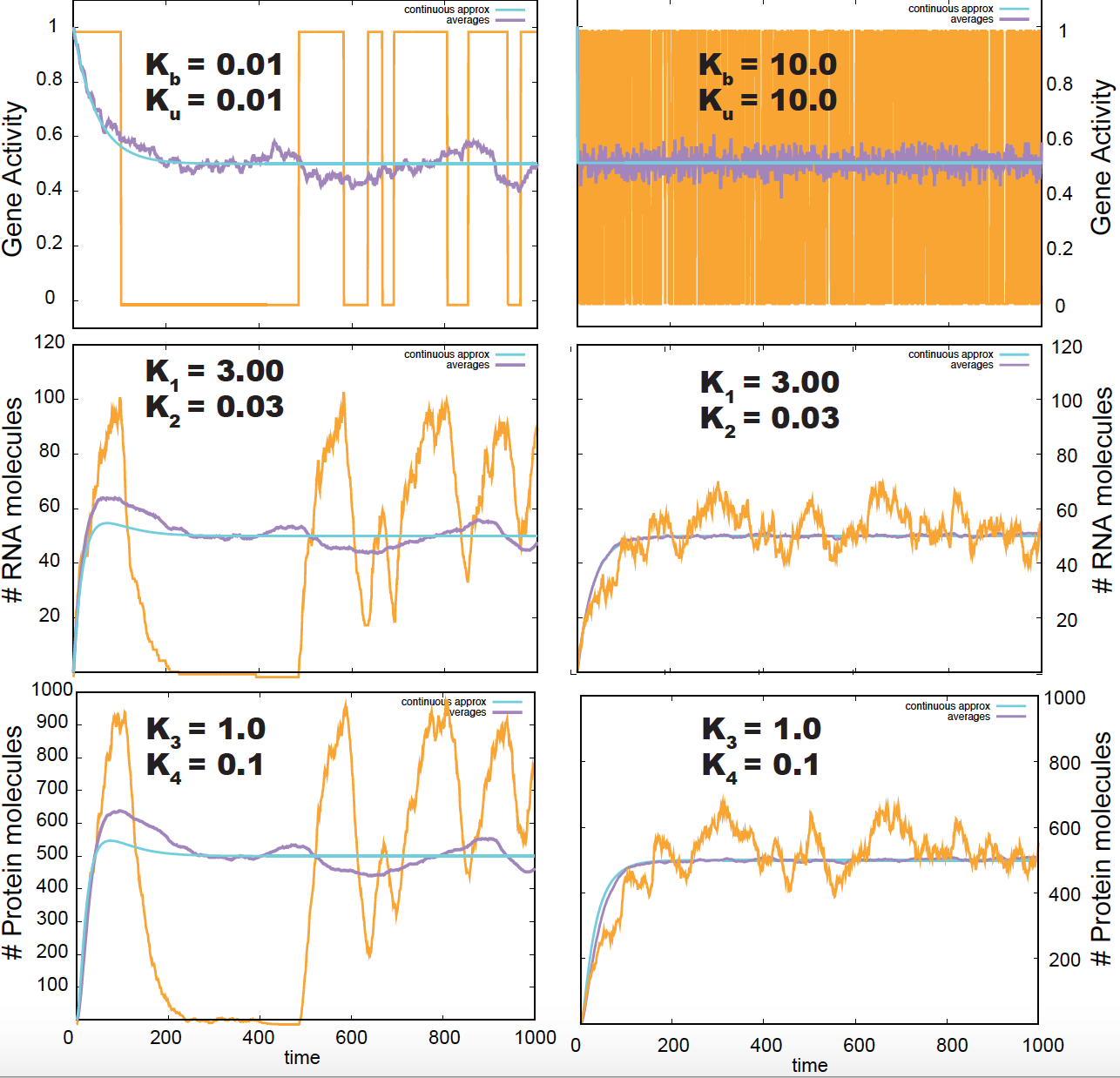
Figure 7. Gillespie simulation of the gene regulation process. In yellow a sampled trajectory, in blue the deterministic solution, in purple the averages of 200 samples.
Resulting in the master equations
\[\begin{aligned} \frac{d P(A, R\mid t)}{d t} = &+ k_b\ P(I, R\mid t) \\ &+ k_1\ P(A, R-1\mid t) \\ &+ k_2\ (R+1)\ P(A, R+1\mid t) \\ &- (k_u + k_1 + k_2 R)\ P(A,R\mid t). \\ \frac{d P(I, R\mid t)}{d t} = &+ k_u\ P(A, R\mid t) \\ &+ k_2\ (R+1)\ P(I, R+1\mid t) \\ &- (k_b + k_2 R)\ P(I, R\mid t) \end{aligned}\]This stochastic system describes a well-known characteristic of transcription, known as transcriptional bursting, which consists on the population of RNA molecules not being stable but experiencing large fluctuations as a function of time.
In this model, when the gene activation/deactivation rates are large, the gene activates and deactivates fast and the RNA population remains quite stable. When the gene activation/deactivation rates are small, the system dwells longer times in either activation (deactivation) state, and the RNA population disappears and reappears in bursts as described in the left panels of Figure 7. Notice that only the stochastic simulations, but not the deterministic solution (in blue) show the bursting phenomena.
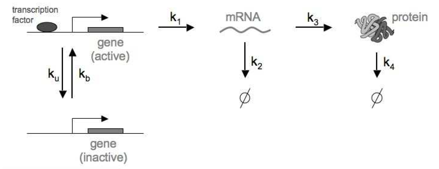
Figure 8. Model that includes regulation of a single gene, transcription and translation, as well as RNA and Protein degradation processes.
RNA and Protein populations from a regulated gene.
In this last example, in addition to gene regulation and RNA production and degradation, we incorporate translation and protein degradation. The reactions (Figure 8) are given by
\[\begin{aligned} \mbox{Gene(I)} &\overset{k_b}{\longrightarrow} \mbox{Gene(A)} \hspace{20mm} \mbox{Gene activation}\\ \mbox{Gene(A)} &\overset{k_u}{\longrightarrow} \mbox{Gene(I)} \hspace{22mm} \mbox{Gene inactivation}\\ \mbox{Gene(A)} &\overset{k_1}{\longrightarrow} \mbox{Gene(A)} + RNA \hspace{5mm} \mbox{RNA synthesis}\\ RNA &\overset{k_2}{\longrightarrow} \emptyset \hspace{34mm} \mbox{RNA degradation}\\ RNA &\overset{k_3}{\longrightarrow} RNA + Protein \hspace{8mm} \mbox{Protein synthesis}\\ Protein &\overset{k_4}{\longrightarrow} \emptyset \hspace{34mm} \mbox{Protein degradation} \end{aligned}\]There are two more reactions in this system (relative to the gene regulation + RNA processing above). The table of reactions and propensities for gene expression is
| r | reaction | propensity | \(\eta(R)\) | \(\eta(P_r)\) |
|---|---|---|---|---|
| 1 | \(\mbox{Gene(I)} \overset{k_b}{\longrightarrow} \mbox{Gene(A)}\) | \(k_b\) | \(0\) | \(0\) |
| 2 | \(\mbox{Gene(A)} \overset{k_u}{\longrightarrow} \mbox{Gene(I)}\) | \(k_u\) | \(0\) | \(0\) |
| 3 | \(\mbox{Gene(A)} \overset{k_1}{\longrightarrow} \mbox{Gene(A)} + RNA\) | \(k_1\) | \(+1\) | \(0\) |
| 4 | \(RNA \overset{k_2}{\longrightarrow} \emptyset\) | \(k_2 R\) | \(-1\) | \(0\) |
| 5 | \(RNA \overset{k_3}{\longrightarrow} RNA + Protein\) | \(k_3 R\) | \(0\) | \(+1\) |
| 6 | \(Protein \overset{k_4}{\longrightarrow} \emptyset\) | \(k_4 P_r\) | \(0\) | \(-1\) |
where \(R\) and \(Pr\) stand for the number of RNA and Protein molecules respectively.
The changes in the joint probability distribution after a small time \(\Delta t\) after allowing at most one reaction in that \(\Delta t\) interval are given by
\[\begin{aligned} P(A, R, Pr\mid t+\Delta t) &=\\ &\begin{array}{rl} + k_b\ \Delta t\ P(I, R, Pr\mid t) & \mbox{change at}\ \Delta t\ \mbox{do to Gene activation reaction}\\ + k_1\ \Delta t\ P(A, R-1, Pr\mid t) & \mbox{change at}\ \Delta t\ \mbox{do to RNA synthesis reaction}\\ + k_2\ (R+1)\ \Delta t\ P(A, R+1, Pr\mid t) & \mbox{change at}\ \Delta t\ \mbox{do to RNA degradation reaction}\\ + k_3 R\ \Delta t\ P(A, R, Pr-1\mid t) & \mbox{change at}\ \Delta t\ \mbox{do to Protein synthesis reaction}\\ + k_4\ (Pr+1)\ \Delta t\ P(A, R, Pr+1\mid t) & \mbox{change at}\ \Delta t\ \mbox{do to Protein degradation reaction}\\ + (1-k_u\Delta t - k_1\Delta t - k_2 R\Delta t - k_3 R\Delta t - k_4 Pr\Delta t)\ P(A, R, Pr\mid t) & \mbox{no change over}\ \Delta t. \end{array}\\ P(I, R, Pr\mid t+\Delta t) &=\\ &\begin{array}{rl} + k_u\ \Delta t\ P(A, R, Pr\mid t) & \mbox{change at}\ \Delta t\ \mbox{do to Gene inactivation reaction}\\ + k_2\ (R+1)\ \Delta t\ P(I, R+1, Pr\mid t) & \mbox{change at}\ \Delta t\ \mbox{do to RNA degradation reaction}\\ + k_3 R\ \Delta t\ P(I, R, Pr-1\mid t) & \mbox{change at}\ \Delta t\ \mbox{do to Protein synthesis reaction}\\ + k_4\ (Pr+1)\ \Delta t\ P(I, R, Pr+1\mid t) & \mbox{change at}\ \Delta t\ \mbox{do to Protein degradation reaction}\\ + (1-k_b\Delta t - k_2 R\Delta t - k_3 R\Delta t - k_4 Pr\Delta t)\ P(I, R, Pr\mid t) & \mbox{no change over}\ \Delta t. \end{array} \end{aligned}\]Resulting in the master equations
\[\begin{aligned} \frac{d P(A, R, Pr\mid t)}{d t} = &+ k_b\ P(I, R, Pr\mid t) - k_u\ P(A,R,Pr\mid t) \\ &+ k_1\ \left[ P(A, R-1, Pr\mid t) - P(A, R, Pr\mid t) \right] \\ &+ k_2\ \left[ (R+1)\ P(A, R+1, Pr\mid t) - R\ P(A, R, Pr\mid t) \right] \\ &+ k_3\ \left[ R\ P(A, R, Pr-1\mid t) - R\ P(A, R, Pr\mid t) \right] \\ &+ k_4\ \left[ (Pr+1)\ P(A, R, Pr+1\mid t) - Pr\ P(A, R, Pr\mid t) \right], \\ \\ \frac{d P(I, R, Pr\mid t)}{d t} = &+ k_u\ P(A, R, Pr\mid t) - k_b P(I, R, Pr\mid t) \\ &+ k_2\ \left[ (R+1)\ P(I, R+1, Pr\mid t) - P(I, R, Pr\mid t) \right] \\ &+ k_3 \left[ R\ P(I, R, Pr-1\mid t) - R\ P(I, R, Pr\mid t) \right] \\ &+ k_4\ \left[ (Pr+1)\ P(I, R, Pr+1\mid t) - Pr\ P(I, R, Pr\mid t) \right]. \end{aligned}\]These differential equations can be solved numerically using the Gillespie algorithm, which I have done (and you will do in the homework and shown results for different parameters in Figure 7. In this figure, I compare several stochastic simulations using the Gillespie algorithm, with the averages of a large number (200) of such simulations (in purple), and with the deterministic solution (in blue).
The conditions under which there is transcriptional bursting (left middle panel in Figure 7), also affect the production of proteins in a similar way (left bottom panel of Figure 7).
The continuous-time differential equations can be obtained with a bit more of algebra the same way we obtained those of the RNA population alone by taking averages over populations.
The continuous-time differential equations and are given by
\[\begin{aligned} \frac{d \langle \mbox{Gene}\rangle_t}{d t} &= k_b - (k_b+k_u)\ \langle \mbox{Gene}\rangle_t \\ \frac{d \langle R\rangle_t}{d t} &= k_1\ \langle \mbox{Gene}\rangle_t - k_2\ \langle R\rangle_t \\ \frac{d \langle P\rangle_t}{d t} &= k_3\ \langle R\rangle_t - k_4\ \langle P\rangle_t. \end{aligned}\]In next week’s lectures, we will see how to obtain these continuous equations for this or any set of reactions, and how to obtain numerical solutions for those equations. The continuous solutions are depicted in Figure 7 in blue, and correspond to the averages of many individual stochastic trajectories.
From the deterministic equations, one can see that the steady is characterized by
\[\begin{aligned} \langle \mbox{Gene}\rangle_{\infty} &= \frac{k_b}{k_b+k_u}\\ \langle R \rangle_{\infty} = \langle \mbox{Gene}\rangle_{\infty}\ \frac{k_1}{k_2} &= \frac{k_b}{k_b+k_u}\ \frac{k_1}{k_2} \\ \langle Pr \rangle_{\infty} = \langle R \rangle_{\infty}\ \frac{k_3}{k_4} &= \frac{k_b}{k_b+k_u}\ \frac{k_1 k_3}{k_2 k_4}\\ \end{aligned}\]