MCB111: Mathematics in Biology (Fall 2024)
week 06:
Probabilistic models and Inference
Preliminars
Present all your reasoning, derivations, plots and code as part of the homework. Imagine that you are writing a short paper that anyone in class should to be able to understand. If you are stuck in some point, please describe the issue and how far you got. A jupyter notebook if you are working in Python is not required, but recommended.
Finding the breakpoints of backcrossed flies
For this homework, we are going to infer the breakpoints of a male fly for which we have mapped reads in a region of 10,000 nucleotides.
The fly is a backcross resulting from a large-scale experiment in which from parents Drosophila Simulans (Dsim) and Drosophila Sechellia (Dsec), F1 hybrid females (Dsec/Dsim) were crossed with Dsec/Dsec parent males.
We also know the sequences of Dsim (\(A\)) and Dsec (\(B\)) for the region of interest, which are giving here.
You should use all the assumptions we make in the w06 lecture, with one simplification. Since we know the Dsim/Dsim ancestry is not possible, we are going to assume only two possible ancestry states
\[\begin{aligned} \mbox{Dsim}&/\mbox{Dsec} = AB, \\ \mbox{Dsec}&/\mbox{Dsec} = BB. \end{aligned}\]Here are some more details about the conditional probabilities that we skipped on the lecture notes.
The model
The \(P(Z_i\mid Z_{i-1})\)
Lets introduce the notation described in Figure 1,
\[P(BB\mid BB) = P(AB\mid AB) = p\]to indicate the probability of staying in the same ancestry.
Let’s assume that due to previous experience with these two Drosophila species, we expect that there is going to be on average one breakpoint (that is a change from homozygous BB to heterozygous AB or viceversa) per chromosome.
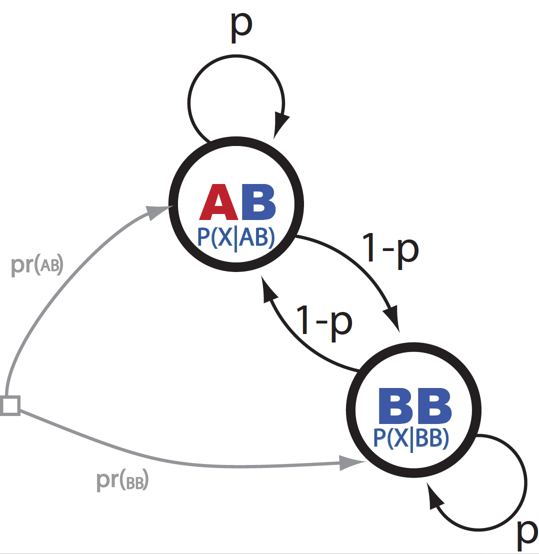
Figure 1. A graphical representation of the HMM.
Our synthetic chromosome has length \(L\), in general, if the number of expected breakpoint is \(n\), then the length of a continuous regions without breakpoints is
\[l = \frac{L}{n+1},\]and because for a geometric distribution
\[l = \frac{p}{1-p}\]then we set the probability of staying in the same ancestry as
\[p = \frac{L/(n+1)}{1+L/(n+1)}\]if we expect \(n\) breaks in a region of length \(L\).
The \(P(X_i \mid G_i)\)
Let’s introduce \(X_i = \{n_a, n_c, n_g, n_t\}\), where \(n_x\) is the count of residue \(x\) in the reads that cover position \(i\).
The conditional probability \(P(X \mid G)\) is a multinomial distribution
\[P(X_i \mid G_i) = \frac{(n_a+n_c+n_g+n_t)!}{n_a! n_c! n_g! n_t!} \left\{ \begin{array}{ll} p_1^{n_a} q_1^{n_c+n_g+n_t} & \mbox{for}\, G_i = aa\\ p_1^{n_c} q_1^{n_g+n_t+n_a} & \mbox{for}\, G_i = cc\\ \ldots & \\ p_2^{n_a+n_c} q_2^{n_g+n_t} & \mbox{for}\, G_i = ac\\ \ldots & \\ \end{array} \right.\]For some Gaussian noise with standard deviation given by \(\epsilon\) and
\[\begin{aligned} p_1 &= 1-\epsilon\\ q_1 &= \frac{\epsilon}{3} \end{aligned}\]and
\[\begin{aligned} p_2 &= \frac{1-\epsilon}{2}\\ q_2 &= \frac{\epsilon}{2}. \end{aligned}\]For this homework, the person who generated the reads tells you that \(\epsilon = 0.4\).
As an example, for locus 10 in Figure 1, we have
\[X_{10} = (5,5,0,0),\]and
\[P(X_{10}\mid G_{10}) = \frac{10!}{5! 5!} \left\{ \begin{array}{ll} p_1^5 q_1^5 & \mbox{for}\, G_{10} = aa, cc\\ q_1^{10} & \mbox{for}\, G_{10} = gg, tt\\ p_2^{10} & \mbox{for}\, G_{10} = ac \\ p_2^5 q_2^5 & \mbox{for}\, G_{10} = ag, at, cg, ct\\ q_2^{10} & \mbox{for}\, G_{10} = gt \end{array} \right.\]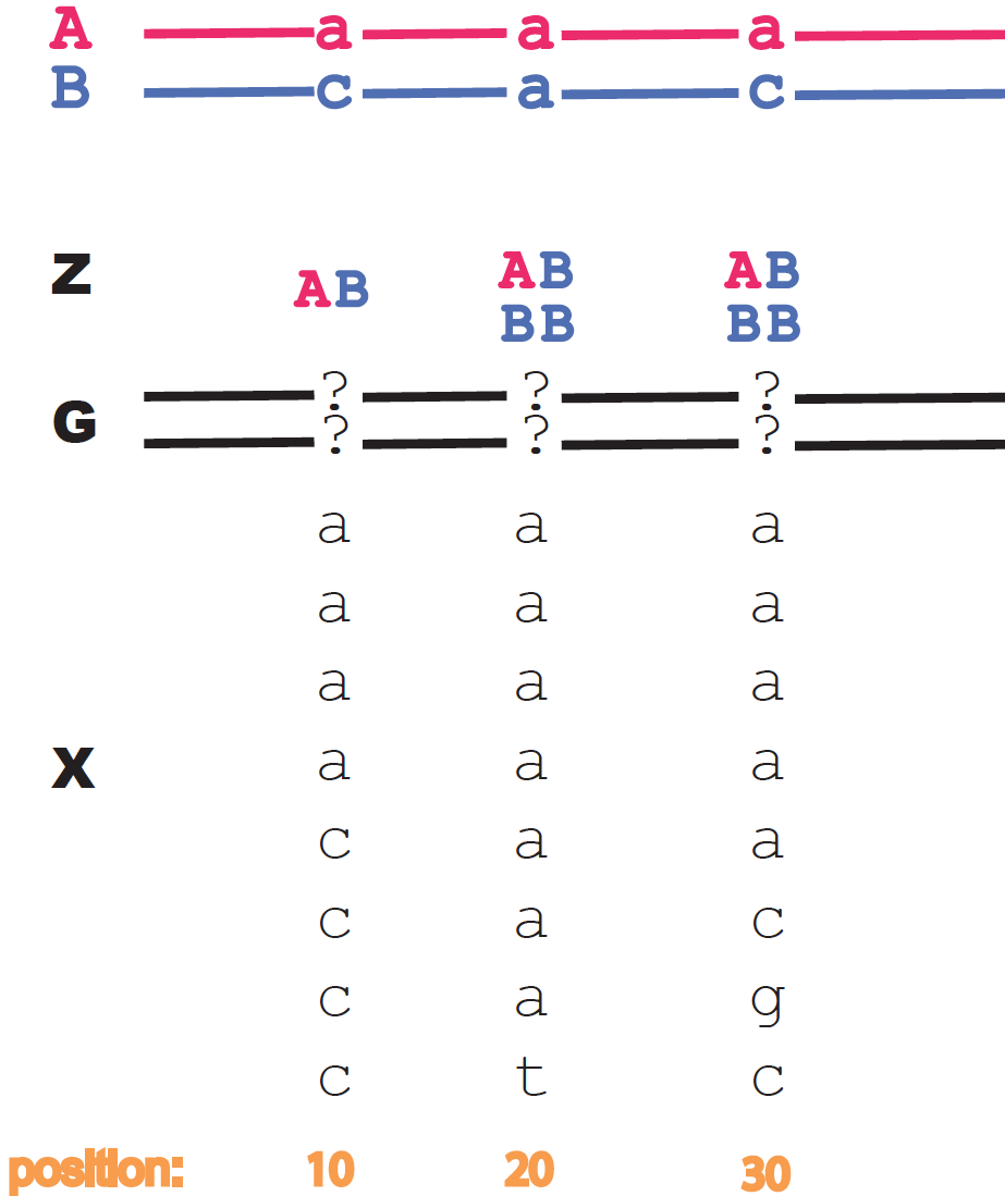
Figure 2. Reads and genome data are given for three hypothetical loci as examples.
The \(P(G_i \mid Z_i)\)
As for the probability of the genotype given the ancestry, we have
\[\begin{aligned} P(G_i \mid BB) &= \left\{ \begin{array}{ll} 1 & G_i=g_i^B g_i^B\\ 0 & \mbox{otherwise} \end{array} \right. \\ P(G_i \mid AB) &= \left\{ \begin{array}{ll} 1 & G_i=g_i^A g_i^B\\ 0 & \mbox{otherwise} \end{array} \right. \end{aligned}\]where \(g^A_i\) is the residue at position \(i\) for strain \(A\), and similarly for \(g^B_i\).
For locus 10 in Figure 1, we have
\[\begin{aligned} P(G_{10} \mid BB) &= \left\{ \begin{array}{ll} 1 & G_{10}=cc\\ 0 & \mbox{otherwise} \end{array} \right. \\ P(G_{10} \mid AB) &= \left\{ \begin{array}{ll} 1 & G_{10}=ac\\ 0 & \mbox{otherwise} \end{array} \right. \end{aligned}\]Andolfatto et al. assume a more general case in which there could be sequencing error, thus a non-zero probability for other genotypes. We have simplified the model and assume no sequencing error at all.
Finally \(P(X_i \mid Z_i)\)
is given by
\[P(X_i \mid Z_i) = \sum_{G_i} P(X_i \mid G_i)\, P(G_i\mid Z_i)\]For locus 10 in Figure 1, we have
\[\begin{aligned} P(X_{10} \mid BB) &= \sum_{G_{10}} P(X_{10} \mid G_{10})\, P(G_{10}\mid BB)\\ &= P(X_{10} \mid cc)\\ &= \frac{10!}{5! 5!}\ p_1^5 q_1^5\\ P(X_{10} \mid AB) &= \sum_{G_{10}} P(X_{10} \mid G_{10})\, P(G_{10}\mid AB)\\ &= P(X_{10} \mid ac)\\ &= \frac{10!}{5! 5!}\ p_2^{10}\\ \end{aligned}\]Since \(q_1\) is an error term, then \(p_2>>q_1\) and \(p_2\approx p_1\), then we have
\[P(X_{10} \mid AB) >> P(X_{10} \mid BB)\]as one would expect by looking at the data in Figure 1.
The data
You are given two files
-
The mapped reads for a region of 10,000 nucleotides.
This file has 10,000 rows, each with four columns. Each column represents the number of As, Cs, Gs, and Ts (in that order) that appeared in all the reads that mapped to that position.
-
The sequence of the genomic regions for the two species “A” and “B”, in fasta format.
Implementation issues
- need to work in logarithms
The forward and backward algorithms require to multiply many small numbers (probabilities). If you try to implement them as multiplications, you will see that soon you run out of precission. Numbers will be so small that you cannot distinguish them.
The solution is to work in logarithm space. Insted of using probabilities, you take the logarithm of the probabilities, and instead of multiplying them you sum them.
So for instance, the first recursion in the forward algorithm
\[f_{AA}(i) = P(X_i\mid AA) \left[ p \, f_{AA}(i-1) + (1-p)\, f_{AB}(i-1) \right]\]becomes
\[\log f_{AA}(i) = \log P(X_i\mid AA) + \log \left[ e^{ \log p+ \log f_{AA}(i-1)} + e^{\log{(1-p)} + \log f_{AB}(i-1)} \right]\]- sum exponentials in a clever way
In the previous expression, we still need to calculate terms of the form
\[\log\left(e^a+e^b\right).\]A numerical trick to keep this quantity in bounds is to find the largest of the two values, say \(a>b\) and to calculate
\[\log\left(e^a+e^b\right) = \log e^a\left(1+e^{b-a}\right) = a + \log{ (1+e^{b-a})}.\]Now the term we are exponentiating is \(b-a<0\) and that exponential is always small.
There are functions both in Matlab and Python that implement this “logsumexp” calculation.
A luxury you will not have in real live
Because this is a simulated experiment, as a control, I can give you information about the actual breakpoints, so that you can check whether your inference is getting the right answer or not.
However, one thing you could do in real live is to generate synthetic data to test your implementation before you deploy your algorithm on real data for which you do not know the real answer.
Because the model we have introduced is probabilistic, for each node, you have defined a probability distribution from which you can sample. A probabilistic model is a generative model. That is how I generated the data for this homework. That is a powerful tool to have.