MCB111: Mathematics in Biology (Fall 2023)
final:
The leaky gated channel
A way to study how a neuron behaves is by studying the activity of its different channels (transmembrane proteins) transporting ions in and out the cell. Using patch clamp techniques, investigators can target an individual channel, and measure its current, that is, the number of ions that go through it during a small time interval.
We are going to look at particular type of channel which transports sodium ions \(Na^{+}\). Increased \(Na^{+}\) inside the cell typically results in an action potential, and lower \(Na^{+}\) corresponds to the neuron being in a resting state.
In a gated channel, the channel has two distinct configurations, open (O) and closed (C). \(Na^{+}\) ions go through the channel when the channel is open, but they are stopped outside the cell when the channel is closed. The open/close mechanism can be controlled many different ways, for instance by changes in voltage (voltage-gated or voltage-sensitive channels), or by binding to a small molecule (the ligand). On the other hand, in a leak channel, the channel is always open.
Here we are going to study a leaky gated channel, that is, a gated channel with defined “open” and “closed” configurations, but such that the channel is somewhat leaky, and that ions can cross even when in the closed state. Mutations showing this phenotype have been found, for instance in this work about calcium channels, “Leaky channels make muscles weak”.
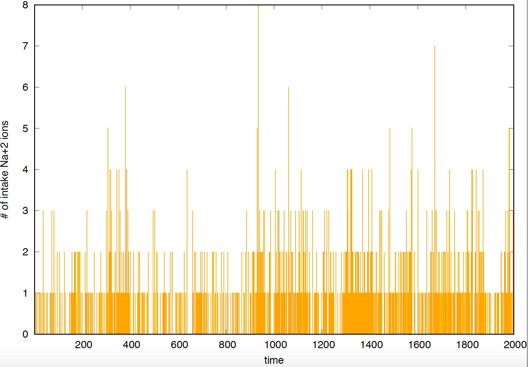
Figure 2. Current observed for a "leaky" gated channel.
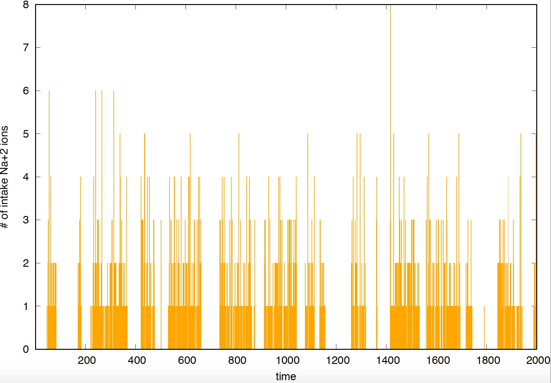
Figure 1. Current observed for a "clean" gated channel.
Using a patch clamp, you can measure the current associated with an individual channel. If the channel opens and closes “cleanly”, that is, ions cross the membrane when the channel is open, but do not when the channel is in the closed configuration, then you would record something like what you see in Figure 1, where it is straightforward to identify when the channel is open and when it is closed. On the other hand, if the channel is leaky, that is, even when the channel is closed some ions can cross the cell membrane, then the current will look like what you see in Figure 2, where it is much harder to identify by eye when the channel was open or closed.
Our goal for this final is to infer when a leaky channel is open and closed by looking at the currents measured by patch clamp.
Deadline: Thursday, Dec 14 at 9:00 am.
The stochastic process
We assume two things
-
In its closed configuration, the channel is leaky, and allows the transport of some ions, hopefully to a lesser extent than the open channel (otherwise the channel would be completely inefficient regulating the amount of \(Na^+\) inside the cell).
-
More than one ion at a time can be transported. If \(k\) is the rate (instantaneous probability) of transporting one ion, then the rate of transporting \(n\) ions is given by \(k^n\). Although only a few atoms will be transported at a given time, in principle the number of possible ions is \(1\leq n \leq \infty\).
According to those assumptions, here are the reactions
\[\begin{aligned} C \overset{k_o}{\longrightarrow} O &\quad\mbox{Channel opens}\\ O \overset{k_c}{\longrightarrow} C &\quad\mbox{Channel closes}\\ O \overset{k_1}{\longrightarrow} O + 1 &\quad\mbox{1 ion crosses inside the cell, when channel is Open}\\ \vdots&\\ O \overset{k_1^n}{\longrightarrow} O + n &\quad\mbox{n ions cross inside the cell, when channel is Open}\\ C \overset{k_2}{\longrightarrow} C + 1 &\quad\mbox{1 ion crosses inside the cell, when channel is Closed}\\ \vdots&\\ C \overset{k_2^n}{\longrightarrow} C + n &\quad\mbox{n ions cross inside the cell, when channel is Closed}\\ \end{aligned}\]where \(k_o\), \(k_c\) \(k_1\) and \(k_2\) are constants. And also,
-
\(N^o\) is the number of \(Na^{+}\) ions outside the cell, which we assume it is very large and approximately constant
-
\(n\) is the number of \(Na^{+}\) ions that go through the channel in \(\Delta t\).
Thus, the probability of a closed channel opening in a small time interval \(\Delta t\) is given by \(k_o \Delta t\), the probability of an open channel letting \(n\) ions through is \(k_1^n \Delta t\), etc.
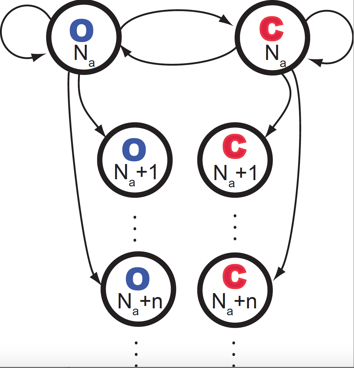
Figure 3. Diagrammatic representation of the leaky channel probabilistic reactions occurring in a small time interval.
Figure 3 describes the different events that can happen in a small time \(\Delta t\). We assume that only one of the possible changes can happen during \(\Delta t\).
The quantity \(N\) (\(N_a\) in Figure 3) represents the current number of \(Na^{+}\) ions inside the cell that have gone through the ion channel after time \(t\). If we use \(n_i\) to refer to the number of ions that cross the channel from \(t_i\) to \(t_i+\Delta t\), then,
\[N(t = m \Delta t) = \sum_{i=1}^{m} n_i.\]-
[Q1.1] Write the probabilities associated to each of the actions (arrows) in Figure 3.
-
[Q1.2] Write the master equations describing the probabilities of the channel being open (\(O\)) or closed (\(C\)) and having \(N\) ions inside the cell at time \(t+\Delta t\), as a function of the distributions at time \(t\).
-
[Q1.3] Often patch recodings measure the total flux in/out the cell through all channel. Assuming all channels are identical, that would give us a recording of the continuous time solution.
Write the continuous-time change of the above distributions
\[\frac{d P(O, N\mid t)}{d t}\\ \frac{d P(C, N\mid t)}{d t}\]which can be derived directly from the master equations.
Hint: remember that for \(k < 1\), then \(\sum_{n=1}^{\infty} k^n = \frac{k}{1-k}\).
Inference of the state of the channel
Another way of representing the system is as given in Figure 4.
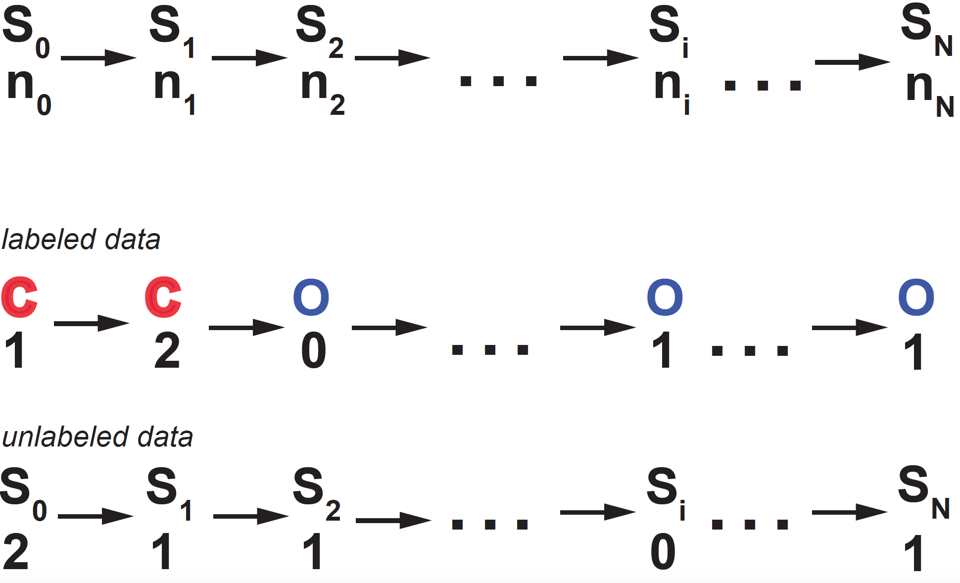
Figure 4. Graphical representation of the leaky-gated channel probabilistic model. At time ti, the channel is at state Si = (O, C), and ni ions come through the channel. Each arrow corresponds to a probability with a unique correspondence to those in Figure 3.
At each time point \(t_i\), there are two random variables: \(S_i\) representing whether the channel is open or closed and \(n_i\) measuring the number of ions that entered the neuron through that channel.
In the actual experiment, you measure the current, that is, the number of ions that went through in that \(\Delta t\), but you don’t know if the channel is open or closed (but still leaking ions inside the cell). At each time point, the state of the channel \(S_i = \{ O\ \mbox{or}\ C\}\) is unknown (a hidden variable).
The results of one experiment are given in file file1. This file includes a list of 400 rows, each with two values: the first column is the time, and the second is the number of \(Na^{+}\) ions that entered the cell through the single channel. The time interval is \(\Delta t = 1\) ms.
\[\begin{array}{lc} t_0 & n_0\\ t_1 = t_0 + \Delta t & n_1\\ t_2 = t_1 + \Delta t & n_2\\ \vdots\\ t_n = t_{n-1} + \Delta t &n_N. \end{array}\]-
[Q2.1] Write the equations that describe the forward and backward algorithms, that calculate the functions
\[f_o(i) \equiv P(n_0, n_1,\ldots, n_i, S_i=O) = \sum_{S_0}\ldots\sum_{S_{i-1}} P(n_0 S_0, n_1 S_1,\ldots, n_i S_i=O)\\ f_c(i) \equiv P(n_0, n_1,\ldots, n_i, S_i=C) = \sum_{S_0}\ldots\sum_{S_{i-1}} P(n_0 S_0, n_1 S_1,\ldots, n_i S_i=C)\] \[b_o(i) \equiv P(n_{i+1},\ldots, n_{N}\mid S_i=O) = \sum_{S_{i+1}}\ldots\sum_{S_{N}} P(n_{i+1} S_{i+1},\ldots, n_N S_N\mid S_i=O)\\ b_c(i) \equiv P(n_{i+1},\ldots, n_{N}\mid S_i=C) = \sum_{S_{i+1}}\ldots\sum_{S_{N}} P(n_{i+1} S_{i+1},\ldots, n_N S_N\mid S_i=C)\]Hint1: Remember to look back at the diagram in Figure 3, in order to figure out how the forward functions \(f_o(i)\) and \(f_c(i)\) depend on \(f_o(i-1)\) and \(f_c(i-1)\), and similarly how the backward functions \(b_o(i)\) and \(b_c(i)\) depend on \(b_o(i+1)\) and \(b_c(i+1)\).
Hint2: Notice that in the interval \(\Delta t\) only one of the possible actions takes place. Then, if in one \(\Delta t\) a channel changes configuration, it cannot in the same time interval let any ions through, or if it lets some ions through, it cannot in the same \(\Delta t\) change configurations. That results in that for instance, \(f_o(i)\) depends on \(f_c(i-1)\) only if at \(t_i\) no ions are transported.
-
[Q2.2] Implement the functions to calculate the forward and backward probabilities for every point. In all implementations assume that \(\Delta t = 1\) ms.
-
[Q2.3] Use the forward and backward functions to calculate the points at which the channel transition from open to closed and viceversa.
For this exercise, you can use the following parameters
\[\begin{aligned} k_o &= 0.012\\ k_c &= 0.014\\ k_1 &= 0.41\\ k_2 &= 0.11 \end{aligned}\]Hint3: If you feel a bit overwhelmed by the many reactions with \(k_1\), \(k_1^2\),… \(k_2\), \(k_2^2\),… Start by considering the case in which only one ion can get througth in a \(\Delta t\) (consider only the \(k_1\) and \(k_2\) reactions). You can get 80% of the credit by solving that simpler case.
Estimation of parameters
You only need to answer one of the two options below for full credit. Extra credit if you answer both.
One obvious weakness of the previous approach is that I had to give you the values of the parameters to use. In real life you do not have that information.
With this question, we explore two ways to getting at what the parameter values may be.
- In the first option, you are not given the values of the parameters, but some extra (and still unrealistic) information about the state of the channel, that is, labeled data.
- In the second option, you are all on your own estimating the parameters from the partial data provided by just knowing the number of ions that go through the channel at each time stamp, but not the state of the channel itself.
[Q3.Opt1] Option 1: Using labeled data
In this case, labeled data means that in addition to knowing the number of ions that get into the cell, you also know the state of the cell \(S\): Open = 1 and Close = 0. In this file2, you can find such data. For each row, there are 4 columns: first is time, second is state of the channel, third is the number of ions that cross, and fourth is the total number of ions up to that time.
-
First, One easy thing you can calculate from labeled data are the dwell times for the channel remaining open and closed.
In the channel open/close exercise in class, the average dwell times had a simple relationship with the rate constants of closing and opening. In this case, those will be slighly modified.
-
Second, you can also easily estimate from the data a histogram for
\[P(\mbox{# ions imported by open channels in the data}\mid k_1),\\ P(\mbox{# ions imported by closed channel in the data}\mid k_2).\]These two empirical distributions are geometric distributions as a function of \(k_1\) AND \(k_2\) respectively.
Using both together you can (just numerically if you want) optimize for \(k_o, k_c, k_1, k_2\).
[Q3.Opt2] Option 2: By expectation-maximization on unlabeled data
You are given again one file, file3, with just the times and number of molecules that enter at that small interval. You should implement the Expectation-Maximization (EM) algorithm to infer the values of all 4 rate constants.
file3 is similar to file1, just with many more measurements of ion intake, as robust optimization of parameters improves with the amount of data at hand.
Remember that EM requires that you calculate expected counts using the current parameters, and then use the expected counts to calculate the new values of the parameters. In this case, we have 4 parameters, but many possible states of the system, e.g., assuming that we have a training set with \(1\leq i\leq N\) measurements:
- Expected number of times the channel goes from \(O\rightarrow C\)
- Expected number of times that an Open channel lets one ion in
- Expected number of times that an Open channel lets two ions in
and so on…
What can we do with so many terms all involving the one parameter \(k_1\) we want to estimate?
Let’s do some marginalization, and consider only 6 cases
- Expectation that the channel goes from \(O\rightarrow C\) (same as above)
- Expectation that any number of ions go through in an Open channel
- Expectation that the channel just remains Open
And the other two “expectations” are
- Expectation that the channel goes from \(C\rightarrow O\)
- Expection that any number of ions go through in an Closed channel
-
Expectation that the channel just remains Closed
\[Cc_3 = \sum_i f_c(i) (1-k_o- \frac{k_2}{1-k_2}) b_c(i+1)\ \delta(n_{i+1}==0)\]
Then, the maximum-likelihood (the maximization step) part of the algorithm that gives you the new estimates of the parameters \(k_o^{(1)}\), \(k_c^{(1)}\), \(k_1^{(1)}\), \(k_2^{(1)}\), are given by
\[\begin{aligned} k_c^{(1)} &= \frac{Co_1}{Co_1+Co_2+Co_3}\\ k_o^{(1)} &= \frac{Cc_1}{Cc_1+Cc_2+Cc_3}\\ \frac{k_1^{(1)}}{1-k_1^{(1)}} &= \frac{Co_2}{Co_1+Co_2+Co_3}\\ \frac{k_2^{(1)}}{1-k_2^{(1)}} &= \frac{Cc_2}{Cc_1+Cc_2+Cc_3}\\ \end{aligned}\]Hint: When proposing initial parameters, remember that all values in Figure 3 have to be probabilities, that is, they cannot take negative values or be larger than one.
Note about notation: the \(\delta(x)\) function is call the Kronecker Delta function, which takes value 1 when the argument is true, and value zero otherwise. In our case, for instance
\[\begin{equation} \delta(n_{i}=0) = \begin{cases} 1 & \mbox{if}\quad n_{i}=0\\ 0 & \mbox{if}\quad n_{i}\neq 0\\ \end{cases} \end{equation}\]or
\[\begin{equation} \delta(n_{i}>0) = \begin{cases} 1 & \mbox{if}\quad n_{i}>0\\ 0 & \mbox{if}\quad n_{i}\leq 0\\ \end{cases} \end{equation}\]