section 07: coin toss expectation maximization
Originally offered as an EM Tutorial by Tim Dunn on 9/30/16
(Based on a primer by Do and Batzoglou)
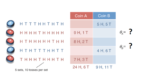
Imagine that you have just observed 5 sets of 10 tosses, where each set was generated by one of the two coins and the identity of the coin used for each set was known. What is the bias on each coin?
As a journeyman Bayesiansmith, you would solve the problem by first setting up an expression for the inverse problem, assuming a uniform prior,
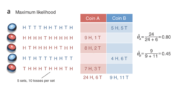
\begin{align} P(\theta_{A} \mid data_{A}) = \frac{P(data_{A} \mid \theta_{A})}{\int_0^1P(data_{A} \mid \theta_{A})\,d\theta_{A}} \\ P(\theta_{B} \mid data_{B}) = \frac{P(data_{B} \mid \theta_{B})}{\int_0^1P(data_{B} \mid \theta_{B})\,d\theta_{B}} \end{align}This would result in a continuous probability density function that carefully expressed your degree of belief in each value of $\theta$, given the observed heads/tails. But what if you only wanted a single, best estimate of $\theta$? How would you guess? For this binomial coin toss, the best guess is the number heads divided by the total number of flips. This maximizes the likelihood of the data and thus represents the maximum likelihood estimates of the paramaters $\theta_{A}$ and $\theta_{B}$.
We can visualize the maximum likelihood by plotting a few points from the likelihood function,
\begin{align} P(H = 24, N = 30 \mid \theta_{A}) = \binom{30}{24}{\theta_{A}}^{24}({1-\theta_{A}})^{6} \end{align}import numpy as np
import matplotlib.pyplot as plt
import scipy.stats as stats
from scipy.special import comb
%matplotlib inline
def likelihood(H, N, points):
return comb(N, H) * np.power(points, H) * np.power(1-points, N-H)
points = np.linspace(0,1,100)
plt.plot(points, likelihood(24, 30, points))
plt.yticks([],[])
plt.xlabel(r'$\theta_{A}$', fontsize=15)
plt.ylabel(r'$P(data \mid \theta_{A})$', fontsize=15)
plt.show()

Note that $\frac{24}{30} = 0.8$
And we can do the same for $\theta_{B}$:
points = np.linspace(0,1,100)
plt.plot(points, likelihood(9, 20, points))
plt.yticks([],[])
plt.xlabel(r'$\theta_{B}$', fontsize=15)
plt.ylabel(r'$P(data \mid \theta_{B})$', fontsize=15)
plt.show()

Note that $\frac{9}{20} = 0.45$
Analytically, we can solve for the maximum likelihood by taking the derivative of the (log) likelihood function. The log form makes our calculation slightly easier, and the max of the log likelihood will occurr at the same vaue of $\theta$ as in the regular likelihood function.
\begin{align} \ln\binom{N}{H}{\theta}^{N}({1-\theta})^{N-H} &= \ln\binom{N}{H} + \ln\theta^{N} + \ln{(1-\theta)}^{N-H} \\ &= \ln\binom{N}{H} + N\ln\theta + (N-H)\ln{(1-\theta)} \end{align}To solve for the maximum, take the derivative with respect to $\theta$, and set it equal to zero,
\begin{align} \frac{d}{d\theta}\ln\binom{N}{H} + N\ln\theta + (N-H)\ln{(1-\theta)} = \frac{N}{\theta} - \frac{N-H}{1-\theta} = 0 \end{align}Solving for $\theta$ gives us $\theta = \frac{H}{N}$, which we denote $\hat{\theta}$.
Expectation Maximization
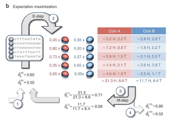
Imagine a similar scenario in which a single coin is chosen for each set, but you are not told which coin was chosen. Without this information, how can you infer the bias on the coins?
First, we need to build a simple graph of the steps taken to generate the data:
\begin{align} choose \ coin \ C \ with \ probability \ p = 0.5 \to flip \ coin \ C \ 10 \ times \ with \ probability \ \theta \to observed \ flips, F \end{align}We can generate data from this model with a simple loop:
theta_a = 0.2
theta_b = 0.6

sets = 5
flips = 10

data = np.zeros((sets, flips))

for i in range(0, sets):
    hidden_theta = np.random.choice([theta_a, theta_b], p=[0.5, 0.5]) # equal probabiltiy of choosing either coin
    for j in range(0, flips): # generate sequences of heads/tails using chosen coin bias. 1 = heads, 0 = tails
        data[i,j] = np.random.choice([1, 0], p=[hidden_theta, 1 - hidden_theta])

data
From the observed flips and the known $\theta$, we can easily calculate the joint probability of the data for every possible set (5) & coin (2),
\begin{align} P(F, C \mid \theta, p) = P(F \mid C, \theta) \times P(C\mid p) \end{align}and marginalize over the different coin possibilities to get $P(F \mid \theta, p)$. Taking the product across $P(F \mid \theta, p)$ from all sets will give us the likelihood of the data given $\theta$.
def coin_likelihood(data, sets, flips, theta_a, theta_b):
    likelihood = 1
    for s in range(0, sets):
        # marginalize across C and multiply across each resulting P(F|theta,p), i.e. set.
        likelihood *= stats.binom.pmf(sum(data[s,:]), flips, theta_a) + stats.binom.pmf(sum(data[s,:]), flips, theta_b)
    return likelihood

coin_likelihood(data, sets, flips, theta_a, theta_b)
But to try to infer some unknown $\theta_{A}$ and $\theta_{B}$, we need to turn the crank of inference using the expectation maximization algorithm. To do this, rather than just calculating the likelihood, we instead calculate the joint probability, $P(F, C \mid \theta, p)$ and normalize by $P(F \mid \theta, p)$, which we calculate using the same marginalization as before. This results in $P(C \mid F, \theta, p)$, which is the probability that a particular coin was flipped (in each set), given the flips and $\theta$.
But wasn't the whole point that we didn't know the true $\theta$? Yes! But we can certainly calculate $P(C \mid F, \theta, p)$ using some estimate of $\theta$.
And why do we care about $P(C \mid F, \theta, p)$ anyway? Well, it gives us the ability to assign some of the heads & tails in each set to each coin. After we've made this weighted assignment, we can calculate a new maximum likelihood for $\theta$ that we can then feed back into $P(C \mid F, \theta, p)$. Magically, when this runs enough times, we converge on a pretty good guess for the real $\theta$ that generated the data.
data = np.array([[1,0,0,0,1,1,0,1,0,1], # data matching the graphic above
                 [1,1,1,1,0,1,1,1,1,1],
                 [1,0,1,1,1,1,1,0,1,1],
                 [1,0,1,0,0,0,1,1,0,0],
                 [0,1,1,1,0,1,1,1,0,1]])

est_theta_a = 0.6 # initial guesses for biases
est_theta_b = 0.5
num_em = 10 # number of EM iterations
track_l = np.zeros((num_em,)) # use to plot the likelihood over EM iterations

for i in range(0,num_em):
    heads_a = 0 # these will store the running tally of heads and tails based on our confidence in each coin
    tails_a = 0
    heads_b = 0
    tails_b = 0
    for s in range(0, sets):
        num_heads = sum(data[s,:])
        num_tails = flips - num_heads
        # by marginalizing over coins, we get our normalization faactor for each set (i.e. row in the table)
        pF = stats.binom.pmf(sum(data[s,:]), flips, est_theta_a) + stats.binom.pmf(sum(data[s,:]), flips, est_theta_b)
        # normalize to get P(C|F,theta,p)
        p_coin_a = stats.binom.pmf(sum(data[s,:]), flips, est_theta_a) / pF
        p_coin_b = stats.binom.pmf(sum(data[s,:]), flips, est_theta_b) / pF

        # use the probabilities to apportion the observed heads and tails to each coin
        heads_a += num_heads * p_coin_a
        heads_b += num_heads * p_coin_b
        tails_a += num_tails * p_coin_a
        tails_b += num_tails * p_coin_b

    # update our estimate of theta
    est_theta_a = heads_a/(heads_a + tails_a)
    est_theta_b = heads_b/(heads_b + tails_b)

    # follow likelihood
    track_l[i] = coin_likelihood(data, sets, flips, est_theta_a, est_theta_b)

plt.plot(track_l,'.-')
plt.xlabel('step #', fontsize=15)
plt.ylabel('likelihood', fontsize=15)
plt.show()

(0.8+0.52)/2
print(est_theta_a) # true value = 0.8
print(est_theta_b) # true value = 0.52