%pylab inline
from IPython.display import clear_output

Populating the interactive namespace from numpy and matplotlib

The materials of this section are borrowed from Prof. Sharad Ramanathan's lecture notes for PHY 286, Mckay's book, Dr. Matthew N. Bernstein's github blog of information theory, and section materials from previous years.

Maximum ignorance/entropy with constraints

Ignorance was related to the probabilities of the different outcomes. If we have a variable x, what probabilities should you assign to each outcome if you are completely ignorant?

If $\sum_{i} p_{i}=1$ is the only constraint (we are completely ignorant), we get an uniform distribution. We expect the probability of each outcome to be equal.

When going from no information at all (except that the probability adds to one) to knowing some information (e.g. mean, variance...), our ignorance decreases, and correspondingly the probabilities we expect for the different outcomes change.

Now let's consider a physical system with different energy levels: $E_1 < E_2 < \dots < E_N$. Consider a single particle in this system that is in a thermal bath and has an average energy E (this is another constraint, or in another word, another piece of information we know about the system). What's the probability that it occupies the energy level $i$.

$\frac{d}{d p_j}\left[-\sum_{i=1}^n p_i \log p_i-\lambda\left(\sum_i p_i-1\right)-\beta\left(\sum_i p_i E_i-E\right)\right]=0 \\ \Longrightarrow p_j=\exp (-1-\lambda) \exp \left(-\beta E_i\right)$

We call $Z=\sum_{i=1}^N \exp \left(-\beta E_i\right)$ as partition function.

$p_i=\frac{1}{Z} \exp \left(-\beta E_i\right)$. From statistical mechanics $\beta =\frac{1}{k_B T}$.

Graphical view of Lagrange multiplier

Maximization of function $f(x,y)$ subject to the constraint $g(x,y)=0$. At the constrained local optimum, the gradients of $f$ and $g$, namely $\nabla f(x,y)$ and $\nabla g(x,y)$, are parallel.

Shannon’s Source Coding Theorem

Digital communication is the transmission of symbolic-valued signals from one place to another. When faced with the problem, for example, of sending a file across the Internet, we must first represent each character by a bit sequence. Because we want to send the file quickly, we want to use as few bits as possible. However, we don't want to use so few bits that the receiver cannot determine what each character was from the bit sequence. For example, we could use one bit for every character: file transmission would be fast but useless because the codebook creates errors. Shannon taught us how much we can compress the data without losing information, what we call today the "Source Coding Theorem".

Suppose we want to transmit a letter with four possible outcomes "A", "B", "C", "D". I'll first encode this letter, transmit the information to you, and you'll decode it. Each of these outcomes has probability:

$p(A)=\frac{1}{2}$, $p(B)=\frac{1}{4}$, $p(C)=\frac{1}{8}$, $p(D)=\frac{1}{8}$.

I want to develop a code for these four outcomes using binary bits (in Morse code we use "dash" and "dot"). One possible way to encode them is:

A = 00, B = 01, C = 10, D = 11

Here I assign the same code length of 2 bits to each outcome. The information being transmitted after encoding is 2 bits.

But notice the entropy/average information of this letter is:

$I=-\sum_i p(i) \log (p(i))=1 / 2 \log (2)+1 / 4 \log (4)+2 / 8 \log (8)=7 / 4$ bits.

We can see that the entropy, or average information of the outcome, is less than two bits. This means that our code is inefficient and is wasting space. It can be compressed.

Another possible way to encode the same four outcomes is:

A = 0, B = 10, C = 110, D = 111

Here the code length (# of bits) assigned to each outcome exactly equals to $-log p_{i}$. The average code length is:

$\bar{l}=p(A) l_A + p(B) l_B + p(C) l_C + p(D) l_D = 7 / 4$ bits.

This code has an expected code length equal to the entropy of this letter that we want to transmit. In fact, this code is maximally compressed.

Given some categorical distribution of random variable X, Shannon’s Source Code Theorem tells us that no matter what code function C you choose, the smallest possible expected code word length is the entropy of X.

$\mathrm{E}[|\mathrm{C}(\mathrm{X})|]=\sum_{\mathrm{x}}|\mathrm{C}(\mathrm{X})| \mathrm{P}(\mathrm{X}=\mathrm{x}) \geq-\sum_{\mathrm{x}} \mathrm{P}(\mathrm{X}=\mathrm{x}) \log \mathrm{P}(\mathrm{X}=\mathrm{x})=\mathrm{H}(\mathrm{X})$

If we know the probability distribution, we can compress the data maximally.

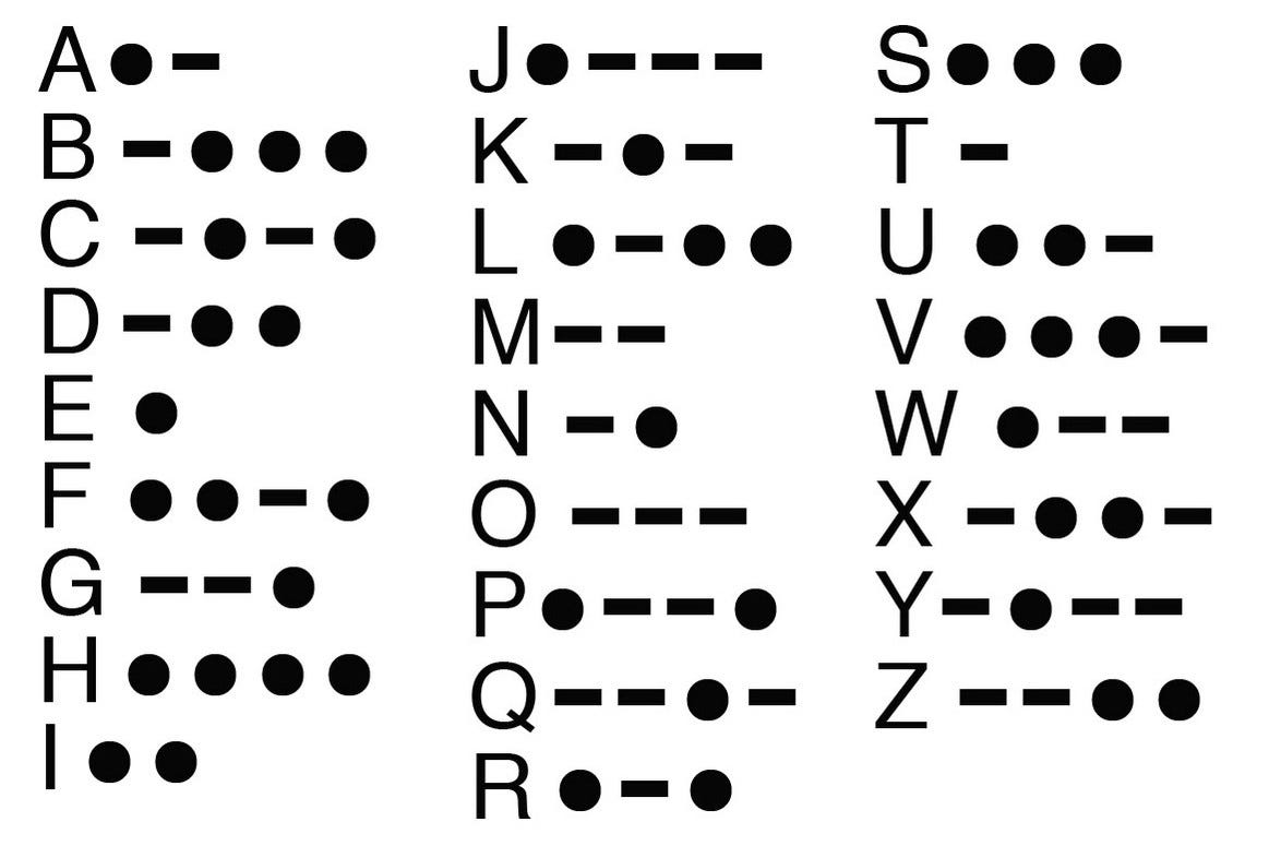
A Morse code, where one assigns a dot for an "e" because it is the most frequent letter of the alphabet.

Mutual information

$ MI(X,Y) = I(X)+I(Y)-I(X,Y)$

import pandas as pd
from IPython.core.display import display, HTML

data1 = {'p(x,y)': ['y=0', 'y=1'],
        'x=0': [0.5, 0],
        'x=1': [0, 0.5]}

df_1 = pd.DataFrame(data1)

df_html_1 = df_1.to_html(index=False)

display(HTML(df_html_1))

p(x,y)	x=0	x=1
y=0	0.5	0.0
y=1	0.0	0.5

$I(X, Y)=-1 / 2 \log (1 / 2)-1 / 2 \log (1 / 2)=1$

$I(X)=I(Y)=-1 / 2 \log (1 / 2)-1 / 2 \log (1 / 2)=1$

$MI(X, Y ) = 1 + 1 − 1 = 1$

The information that knowledge of variable X gives about variable Y is 1 bit. This is equal to the amount of information stored in variable Y alone. Therefore, X tells us everything about Y and vice versa.

data2 = {'p(x,y)': ['y=0', 'y=1'],
        'x=0': [0, 0.5],
        'x=1': [0, 0.5]}

df_2 = pd.DataFrame(data2)

df_html_2 = df_2.to_html(index=False)

display(HTML(df_html_2))

p(x,y)	x=0	x=1
y=0	0.0	0.0
y=1	0.5	0.5

$I(X, Y)=-1 / 2 \log (1 / 2)-1 / 2 \log (1 / 2)=1$

$I(X)=-1 / 2 \log (1 / 2)-1 / 2 \log (1 / 2)=1$

$I(Y)=0$

$MI(X, Y ) = 1 + 0 − 1 = 0$

If we know the value of Y, we have still gained zero information about the value of X. Similarly, if we know the value of X, we have still gained zero information about the value of Y (since there was already only one possibility).

$M(X, Y) \\ =-\sum_{x} p(x) \log (p(x))-\sum_{y} p(y) \log (p(y))+\sum_{x, y} p(x, y) \log (p(x, y)) \\ =-\sum_{x, y} p(x, y) \log (p(x))-\sum_{x, y} p(x, y) \log (p(y))+\sum_{x, y} p(x, y) \log (p(x, y))\\ =\sum_{x, y} p(x, y) \log \left(\frac{p(x, y)}{p(x) p(y)}\right)$

The mutual information is the Kullback-Leibler distance between two distributions $p(x,y)$ and $p(x)p(y)$.

$M(X, Y) \\ =I(x)-[-\sum_{x,y} p(x,y) \log (p(x|y))] \\ =I(x)-[-\sum_{y} p(y) \sum_{x} p(x|y) \log (p(x|y))]\\ =I(x)-I(x|y)\\ =I(y)-I(y|x)$

$I(x|y)$ is the ignorance/entropy of x given y. Mutual information is the reduction in ignorance of X once you know Y.

Information content of DNA sequences

Often in the field of bioinformatics a question comes to mind: What is the shortest (motif) that we expect to appear only once? or What is the shortest length that can be uniquely found in the genome?

This is important to find out when you are trying to figure out if a DNA sequence of interest is appearing in a genome simply by chance or it is a significant appearance.

Eukaryotic genomes have on the order of L=$10^6−10^{10}$ nucleotides. We can define $l$, an arbitrary length of a motif of interest. We can also begin by saying that the composition of different bases (A, C, G, T) is balanced such that we have equal amounts of each throughout the genome.

Let's generate a function that generates genomes with predetermined characteristics, so we can test some of these concept empirically:

def generate_genome(size, g_content, c_content, a_content):

  '''
  This function generates a genome of user defined size and GC content.

  Parameters:
    - Number of bases.
    - % of GC content.
  '''

  g_comp = ['G']*g_content
  c_comp = ['C']*c_content
  a_comp = ['A']*a_content
  t_comp = ['T']*(100-(g_content+c_content+a_content))

  human_genome_composition = np.array(g_comp+a_comp+t_comp+c_comp) # making array with target composition
  human_genome = np.random.choice(human_genome_composition, int(size)) # sampling from composition to generate full genome.

  return ''.join(human_genome) # returns dull genome string form

 %%time
 genome = generate_genome(size = 10e6, g_content = 25, c_content = 25, a_content=25)

genome[:20]

bases , counts =  np.unique(list(genome), return_counts=True)
comps = counts/10e6*100

print("Composition of our mock genome:\n"
        + bases[0]+": " + str(round(comps[0],2)) + " %\n"
        + bases[1]+": " + str(round(comps[1],2)) + " %\n"
        + bases[2]+": " + str(round(comps[2],2)) + " %\n"
        + bases[3]+": " + str(round(comps[3],2)) + " %" )

Now we can play with our genome. For instance if we pick our motif to be “A”, it is expected to land in 1/4 of the positions in the genome. ~2.5M times

genome.count('A')

If we take a motif of length l=2, for instance “AA” it will match fewer than 1/4, but not much better. ~0.5M times

s = 'AAAA'

s.count('AA')

genome.count('AA')

We kindof see a pattern here, the longer the sequence the less it is likely to be found in the genome. Lets try to build an intuition for the information content of a sequence by following a series of thought experiments that we can then validate through code.

First Let's imagine we have a genome with 50% G, 50% C and 0% A or T composition when we sample from it sequentially, we know that we are only going to get Gs and Cs

How surprised would we be if the next sample that we took was either a G or a C? not much, right? Because these are the only two possibilitties in this example. If we expect a G or a C with a 50% chance we would be equally surprised if we got one or the other.

However, it is hard to say how surprised we would be (infinitely?) if the next sample was an A or a T. So it really isn't well defined but that's ok because we are talking about events that can't happen.

genome = generate_genome(size = 1000, g_content = 50, c_content = 50, a_content=0) #Make genome size manageable for dynamic plotting.
As = 0
Ts = 0
Gs = 0
Cs = 0

while (As+Ts+Gs+Cs)<=200:

    clear_output(wait=True)
    fig,ax = subplots(ncols= 1,nrows =1, sharey = False)
    ax.bar(['A','C','T','G'],[As,Cs,Ts,Gs])
    ax.set_xlabel('Nucleotide')
    ax.set_ylabel('Count')
    sample = np.random.choice(list(genome),1) # making the string genome a list to sample easily

    if sample == 'C':
        Cs += 1
    if sample == 'T':
        Ts += 1
    if sample == 'G':
        Gs += 1
    if sample == 'A':
        As += 1
    plt.show()

Lets now see what happens if make the genome 90% GC (45 and 45) and 10% AT (5 and 5).

genome = generate_genome(size = 1000, g_content = 45, c_content = 45, a_content=5) #Make genome size manageable for dynamic plotting.
As = 0
Ts = 0
Gs = 0
Cs = 0

while (As+Ts+Gs+Cs)<=200:

    clear_output(wait=True)
    fig,ax = subplots(ncols= 1,nrows =1, sharey = False)
    ax.bar(['A','C','T','G'],[As,Cs,Ts,Gs])
    ax.set_xlabel('Nucleotide')
    ax.set_ylabel('Count')
    sample = np.random.choice(list(genome),1) # making the string genome a list to sample easily

    if sample == 'C':
        Cs += 1
    if sample == 'T':
        Ts += 1
    if sample == 'G':
        Gs += 1
    if sample == 'A':
        As += 1
    plt.show()

This example basically shows us that surprise is inversely related to probability, the more likely an event is to occur the less surprised we'll be if it actually occurs and vice-versa.

In other words and specifically for our example if the probability of sampling an A or an T is low, the surprise of sampling either is high. And if the probability of sampling an C or an G is high, the surprise of sampling either is low.

A good way to describe this mathematically is by taking the logarithm of the inverse of the probability:

$$\mbox{Surprise}= S = \log{\frac{1}{p(x)}}$$

In that case we could calculate the amount of surpise we'd expect for our genomes, for this last case it would be:

\begin{aligned} S_{A} &= \log{\frac{1}{p(A)}} = \log{\frac{1}{0.05}} \approx 3 \\ S_{T} &= \log{\frac{1}{p(T)}} = \log{\frac{1}{0.05}} \approx 3 \\ S_{C} &= \log{\frac{1}{p(C)}} = \log{\frac{1}{0.45}} \approx 0.8 \\ S_{G} &= \log{\frac{1}{p(G)}} = \log{\frac{1}{0.45}} \approx 0.8 \end{aligned}

As expected the surprise of sampling a G or a C is smaller than it is for an A or a T.

But what about longer motifs? Let's say we want to know the probability of finding the sequence GGA, well then the probability of getting an G $p(G) = 0.45$ and the probability of getting an A $p(A) = 0.05$, so the probability of getting the motif is:

$$p(GGA) = p(G) \times p(G) \times p(A) = 0.45 \times 0.45 \times 0.05 \approx 0.01 $$

If we want to know exactly how surprising it would be so observe this particular we can plug this probability in our previous expression for surprise:

$$S_{GGA} = \log{\frac{1}{p(GGA)}} = \log{\frac{1}{0.01}} \approx 4.59$$

But more importantly notice that the total surprise for the motif is the sum of individual surprises (because of the properties of logarithms.)

$$S_{GGA} = \log{\frac{1}{p(G)}} + \log{\frac{1}{p(G)}} + \log{\frac{1}{p(A)}} = \log{1} - (log{G} + log{G} + log{A}) \approx 4.59$$

So far we have been talking about surprise and this must feel familiar after this weeks class. That is because entropy (E) is the average surprise per event.

Tying this back to our example, how can we calculate the average entropy of a motif of length $l$?

Let's first look at the entropy at a single position, which is one base of the possible A, G, C, T.

$$E_\mbox{position} = \sum_{base \in \{A, G, C, T \} } p(base) \times surprise_{base}$$

Plugging in what we set as the surprise, and simplifying:

$$E_\mbox{position} = -\sum_{base \in \{A, G, C, T \} } p(base) \times \log p(base)$$ Assuming positions are independent of each other, we can use the additivity property of entropy to calculate the entropy of a motif of length $l$:

$$E_\mbox{motif} = l \times E_\mbox{position} = -l \big(\sum_{base \in \{A, G, C, T \} } p(base) \times \log p(base) \big)$$ We've arrived at the formula described by shannon for entropy. What this tells us is the average information content per base position. It turns out there's a very concrete interpretation for this: it measures number of bits in a given message.

- But how can we address the original question we had in mind? (see top of the notebook if you've forgotten already.)

Let's try to tackle this question using the concept of Entropy. And for simplicity we are going to assume from now on that bases in the genome have equal probabilities of occurring along the genome.

The entropy of the location of a motif is going to depend on how many times we can fit the available positions of the genome, for large (or circular) genomes of length $L$ the length of the motif $l$ is usually negligible and we can think of the number of times that we can fit the length of the motif in the genome to be the number of bases in the genome. Let $X$ be a discrete random variable representing the location in a genome of length $L$ (i.e. position 1, 2, ... $L$).

An expression for the entropy of the location in the genome can be written as follows:

$$E_\mbox{location} = -\sum_{i=1}^{L} p(x_i) \log(p(x_i)) $$

Let's assume all locations of the genome are equally likely for the motif, so the probability of finding the motif at any $x_i$ is:

$$p(x_i) = \frac{1}{L} $$

Plugging this back into the equation we get:

$$E_\mbox{location} = - \log(1/L) $$

$$E_\mbox{location} = \log(L) $$

We can also calculate the information content of our motif:

$$E_\mbox{motif} = -l \big(\sum_{base \in \{A, G, C, T \} } p(base) \times \log p(base) \big)$$

Let's assume that A, G, C, T are all equally likely, so we have a $p(A) = p(G) = p(C) = p(T) = 1/4$:

$$\begin{aligned} E_\mbox{motif} &= -l \big(\sum_{base \in \{A, G, C, T \} } \frac{1}{4} \times \log \frac{1}{4} \big) \\ &= -l \log \frac{1}{4} \\ &= l \log 4 \\ & = 2l \\ \end{aligned}$$

Great, now what we want is to find the $l$ so that the entropy of our motif is at least as large as the entropy of the location:

$$\begin{aligned} E_\mbox{location} &\leq E_\mbox{motif} \\ \log L &\leq 2l \\ \end{aligned}$$

Thus: $$ l \geq \frac{1}{2}log(L) $$

The sequence has to be at least $\frac{1}{2}log(L)$ long for it to be in a genome with equal base composition. We can check this computationally!

Let's generate genomes of size $10\times10^6$ which means that the minimum sequence length for it to be uniquely found in a genome of that size must be at least 12 bases long (rounding up!). Let's make 10 genomes to sample from. and pick a couple of length 12 motifs to see how many times they come up in the genomes:

L = 10e6
1/2 * np.log2(L)

%%time
genomes = [generate_genome(size = 10e6, g_content = 25, c_content = 25, a_content=25) for g in range(10)]
motifs_16 = [generate_genome(size=16, g_content = 25, c_content = 25, a_content=25) for g in range(1000)]
motifs_12 = [generate_genome(size=12, g_content = 25, c_content = 25, a_content=25) for g in range(1000)]
motifs_11 = [generate_genome(size=11, g_content = 25, c_content = 25, a_content=25) for g in range(1000)]
motifs_9 = [generate_genome(size=9, g_content = 25, c_content = 25, a_content=25) for g in range(1000)]

counts_16 = [[genome.count(motif) for motif in np.random.choice(motifs_16,100)] for genome in genomes]
print('100 motifs of length 16 appear, on average ' + str(mean(counts_16)) + u" \u00B1 " + str(round(std(counts_16),2)))

counts_12 = [[genome.count(motif) for motif in np.random.choice(motifs_12,100)] for genome in genomes]
print('100 motifs of length 12 appear, on average ' + str(mean(counts_12)) + u" \u00B1 " + str(round(std(counts_12),2)))

counts_11 = [[genome.count(motif) for motif in np.random.choice(motifs_11,100)] for genome in genomes]
print('100 motifs of length 11 appear, on average ' + str(mean(counts_11)) + u" \u00B1 " + str(round(std(counts_11),2)))

counts_9 = [[genome.count(motif) for motif in np.random.choice(motifs_9,100)] for genome in genomes]
print('100 motifs of length 9 appear, on average ' + str(mean(counts_9)) + u" \u00B1 " + str(round(std(counts_9),2)))