week 10:

Molecular Population Dynamics as a Markov Process

Stochastic simulation of transcriptional bursting

Sampling fast from an exponential distribution

In the Gillespie algorithm, dwell times \(\tau\) follow a exponential distribution.

The probability density function (PDF) is

\[PDF(t) = W_R e^{-W_R\ t}.\]

In order to sample a dwell time \(\tau\), we used the cumulative probability function (CDF)

\[CDF(\tau) = \int_0^{\tau} W_R\ e^{-W_R\ t}\ dt\]

such that for a random number \(0\leq x\leq 1\), the sampled dwell \(\tau\) time is given by

\[x = CDF(\tau).\]

The CDF of the exponential distribution has a closed form given by

\[CDF(\tau) = \int_0^{\tau} W_R\ e^{-W_R\ t} = 1 - e^{-W_R\ \tau}.\]

Then, the sampled time is given by

\[\tau = -\frac{1}{W_R}\ \log(1-x).\]

If \(x\) is a random number in \([0,1]\), then \(1-x\) is also a random number in the same range, then we can take the sampled dwell time \(\tau\) given by

\[\tau = -\frac{1}{W_R}\ \log(x).\]

Implementing the Gillespie algorithm

For the stochastic process described in Figure 1, the reactions are given by

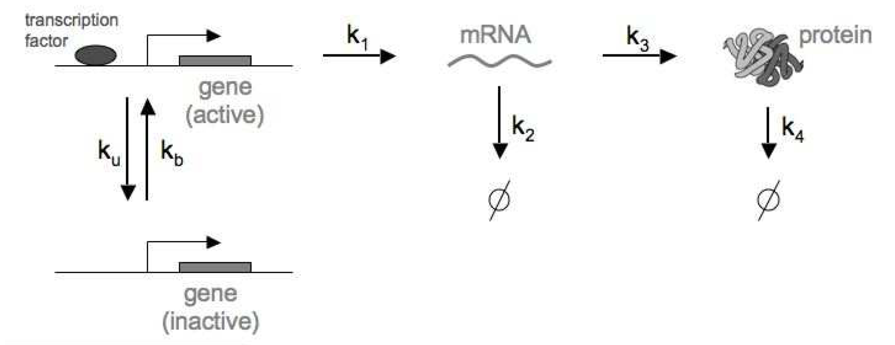
Figure 1. Regulation of a single gene, transcription and translation, as well as RNA and Protein degradation processes.

r	reaction	propensity \(w_r\)	\(\eta(R)\)	\(\eta(P)\)
1	\(\mbox{Gene(I)} \overset{k_b}{\longrightarrow} \mbox{Gene(A)}\)	\(k_b\)	\(0\)	\(0\)
2	\(\mbox{Gene(A)} \overset{k_u}{\longrightarrow} \mbox{Gene(I)}\)	\(k_u\)	\(0\)	\(0\)
3	\(\mbox{Gene(A)} \overset{k_1}{\longrightarrow} RNA\)	\(k_1\)	\(+1\)	\(0\)
4	\(RNA \overset{k_2}{\longrightarrow} \emptyset\)	\(k_2 R\)	\(-1\)	\(0\)
5	\(RNA \overset{k_3}{\longrightarrow} Protein\)	\(k_3 R\)	\(0\)	\(+1\)
6	\(Protein \overset{k_4}{\longrightarrow} \emptyset\)	\(k_4 P\)	\(0\)	\(-1\)

Then the Gillespie algorithm works as follows

Initialize at \(t = 0\),
\[\begin{aligned} Gact &= 1,\\ R &= 0,\\ P &= 0.\\ \end{aligned}\]
Keep a current count of \(t\), \(Gact\), \(R\) and \(P\).
- \(Gact = 1\) if the gene is active (A) at time \(t\), or
- \(Gact = 0\) if the gene is inactive (I) at time \(t\).
- \(R\) is the number of RNA molecules at time \(t\).
- \(P\) is the number of protein molecules at time \(t\).
Sample a dwell time \(\tau\) from a exponential distribution
\[W_R\ e^{-W_R\ t},\]
where the total propensity is given by
\[\begin{aligned} W_R = w_1 + w_4 + w_5 + w_6,\quad &\mbox{if}\, Gact = 0,\\ W_R = w_2 + w_3 + w_4 + w_5 + w_6,\quad &\mbox{if}\, Gact = 1.\\ \end {aligned}\]
Update the current time \(t\) as

\[t\rightarrow t+\tau.\]

Sample one reaction \(r\) according to their propensities
\[P(r) = \frac{w_r}{W_R}.\]
Update \(Gact\), \(R\) and \(P\)
- If \(r = 1\), then \(Gact=0 \rightarrow 1\)
- If \(r = 2\), then \(Gact=1 \rightarrow 0\)
- If \(r = 3\), then \(R \rightarrow R+1\)
- If \(r = 4\), then \(R \rightarrow R-1\)
- If \(r = 5\), then \(P \rightarrow P+1\)
- If \(r = 6\), then \(P \rightarrow P-1\)
Update the propensities according to the new values of \(Gact\), \(R\) and \(P\).
Go back to sampling a new dwell time, until a maximum time \(T\).