MCB111: Mathematics in Biology (Fall 2024)
week 08:
Neural Networks - Learning as Inference
Motivation for the logistic function
The logistic function appears in problems where there is a binary decision to make. Here you will workout a problem (based on MacKays’s exercise 39.5) that like a binary neuron, also uses a logistic function.
The noisy LED display
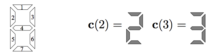
Figure 1. The noisy LED. Figure extracted from MacKay's Chapter 39.
In a LED display each number corresponds to a pattern of on(1) or off(0) for the 7 different elements that compose the display. For instance, the patterns for numbers 2 and 3 are:
\[\mathbf{c}(2) = (1,0,1,1,1,0,1)\] \[\mathbf{c}(3) = (1,0,1,1,0,1,1)\]Imagine you have a LED display that is not working properly. This defective LED is such that, for a given number the LED wants to display:
-
Elements that have to be off, are wrongly on with probability \(f\).
-
Elements that have to be on, are actually on with probability \(1-f\),
The LED is allowed to display ONLY a number “2” or a number “3”. And it does so by emitting a patter \(\mathbf{p}=(p1,p2,p3,p4,p5,p6,p7)\), where \(p_i = 1,0\)
Calculate the posterior probability that the intended number was a “2”, given the pattern \(\mathbf{p}\) you observe in the LED, that is,
\[P(n=2\mid \mathbf{p}).\]Show that you can express that posterior probability as a logistic function,
\[P(n=2\mid \mathbf{p}) = \frac{1}{1+e^{-\mathbf{w}\mathbf{p} + \theta}}\]for some weights \(\mathbf{w}\), and some constant \(\theta\).
You can assume that the prior probabilities for either number, \(P_2\) and \(P_3\), are given.
Hint: \(x^y = e^{y\log x}\) for any two real numbers \(x, y\).
Solution
The probability that we can calculate is \(P(\mathbf{p}\mid 2)\), that is the probability that observing a particular pattern \(\mathbf{p}\), given that the LED tried to emit a “2”,
\[P(\mathbf{p}\mid 2) = (1-f)^{p_1+p_3+p_4+p_5+p_7}\, f^{p2+p_6}.\]Using vector notation,
\[P(\mathbf{p}\mid 2) = (1-f)^{\mathbf{c}(2)\mathbf{p}}\, f^{\mathbf{\hat c} (2)\mathbf{p}},\]where
\[{\hat c}(2)_i = 1- c(2)_i.\]Then using the hint above, we can rewrite,
\[\begin{aligned} P(\mathbf{p}\mid 2) &= e^{\log(1-f)\mathbf{c}(2)\,\mathbf{p}}\, e^{\log(f)\,\mathbf{\hat c} (2)\mathbf{p}}\\ &= e^{\log(1-f)\,\mathbf{c}(2)\mathbf{p} + \log(f)\,\mathbf{\hat c} (2)\mathbf{p}}\\ &= e^{\left[\log(1-f)\,\mathbf{c}(2) + \log(f)\,\mathbf{\hat c} (2)\right]\mathbf{p}}.\\ \end{aligned}\]Introducing the vector
\[\mathbf{a}(2) = \log(1-f)\,\mathbf{c}(2) + \log(f)\,\mathbf{\hat c} (2)\]such that
\[a(2)_i = \log(1-f)\,c(2)_i + \log(f)\,\left(1-c(2)_i\right),\]we can write with all generality
\[P(\mathbf{p}\mid 2) = e^{\mathbf{a}(2)\,\mathbf{p}}.\]The quantity we have been asked to calculate is not \(P(\mathbf{p}\mid 2)\), but instead, given that we have seen a pattern \(\mathbf{p}\), what is the probability that the pattern was generated with a “2” in mind. That is the posterior probability \(P(2\mid \mathbf{p})\), which using Bayes theorem is given as a function of \(P(\mathbf{p}\mid 2)\) as
\[P(2\mid \mathbf{p}) = \frac{P(\mathbf{p}\mid 2) P(2)}{P(\mathbf{p})},\]where \(P(2)\) is a prior probability.
In the general case in which the LED can produce any of the 10 digits (from 0 to 9), then we have by marginalization
\[\begin{aligned} P(\mathbf{p}) &= P(\mathbf{p}\mid 0) P(0) + P(\mathbf{p}\mid 1) P(1) + P(\mathbf{p}\mid 2) P(2) + \ldots + P(\mathbf{p}\mid 9) P(9)\\ &= \sum_{n=0}^{9} e^{\mathbf{a}(n)\,\mathbf{p}}\, P(n). \end{aligned}\]Resulting in the general solution,
\[P(2\mid \mathbf{p}) = \frac{e^{\mathbf{a}(2)\,\mathbf{p}}\, P(2)}{\sum_{n=0}^{9} e^{\mathbf{a}(n)\,\mathbf{p}}\, P(n)},\]Notice that, the normalization condition is \(\sum_{n=0}^9 P(n\mid \mathbf{p}) = 1\).
For our particular problem, where we want to distinguish only between the pattern being generated by a “2” or a “3”, that results in
\[P(2\mid \mathbf{p}) = \frac{e^{\mathbf{a}(2)\,\mathbf{p}}\, P(2)}{e^{\mathbf{a}(2)\,\mathbf{p}}\, P(2) + e^{\mathbf{a}(3)\,\mathbf{p}}\, P(3)},\]where here the normalization condition is
\[P(2\mid \mathbf{p}) + P(3\mid \mathbf{p}) = 1.\]The posterior probability \(P(2\mid \mathbf{p})\) can be re-written as
\[P(2\mid \mathbf{p}) = \frac{1}{1 + e^{\left[\mathbf{a}(3)-\mathbf{a}(2)\right]\,\mathbf{p}}\, \frac{P(3)}{P(2)}}.\]We can define the weights
\[\mathbf{w} = \mathbf{a}(3)-\mathbf{a}(2).\]We can also parameterize the priors as
\[\frac{P(3)}{P(2)}=e^\theta.\]For instance, \(\theta = -\log(2)\) for \(P(2) = P(3) = 1/2\).
Then, we have the expression we wanted to obtain of \(P(2\mid \mathbf{p})\) as a logistic linear function
\[P(2\mid \mathbf{p}) = \frac{1}{1 + e^{\mathbf{w}\,\mathbf{p} + \theta}},\]with weights,
\[\begin{aligned} w_i &= a(3)_i - a(2)_i\\ &= \log(1-f)\,\left[c(3)_i - c(2)_i\right] + \log(f)\,\left[c(2)_i - c(3)_i\right]\\ &=\frac{\log(1-f)}{\log f}\left[c(3)_i-c(2)_i\right]\\ \end{aligned}\]or
\[\mathbf{w} = \frac{\log(1-f)}{\log f}\left(0, 0, 0, 0, -1, 1, 0\right).\]