MCB111: Mathematics in Biology (Fall 2024)
week 00:
The purpose of our homework this week is to develop intuition for measurements resulting from different probability distributions. When values are recorded that obey some fundamental distribution, we want an idea of what they will look like. We would also like to have a sense of how many samples it takes to identify the underlying distribution with some confidence.
Sampling from a distribution
Sampling from the distribution is similar to randomly throwing a dart at the distribution, and recording the x-coordinate of where it struck. For example, with the Gaussian distribution, we can expect to find the darts strike most frequently near the average value (the center of the distribution). Meanwhile, darts hit the uniform distribution evenly at all x-coordinates.
How can we achieve this sort of sampling with a simple computer script? Conveniently you can directly sample from distributions with Python functions such as: numpy.random, scipy.stats.expon, or scipy.stats.norm.
However, the goal here is that you do it yourself just using only the rand() function, so you understand what is going on, and pay attention to the implementation details.
Algorithm for discrete sampling using only the random() function
So we said that sampling a probability distribution is like throwing darts that land randomly somewhere under its curve. How can we accomplish this if we can only “throw darts” uniformly between 0 and 1?
Consider the exponential distribution, we are much more likely to hit a dart close to the value 0 than some value much past our mean. The \(x\) values corresponding to higher probability values span more space for our dart to land, so they are over-represented. This translates directly to the cumulative distribution function (exponential CDF: second figure on the right https://en.wikipedia.org/wiki/Exponential_distribution).
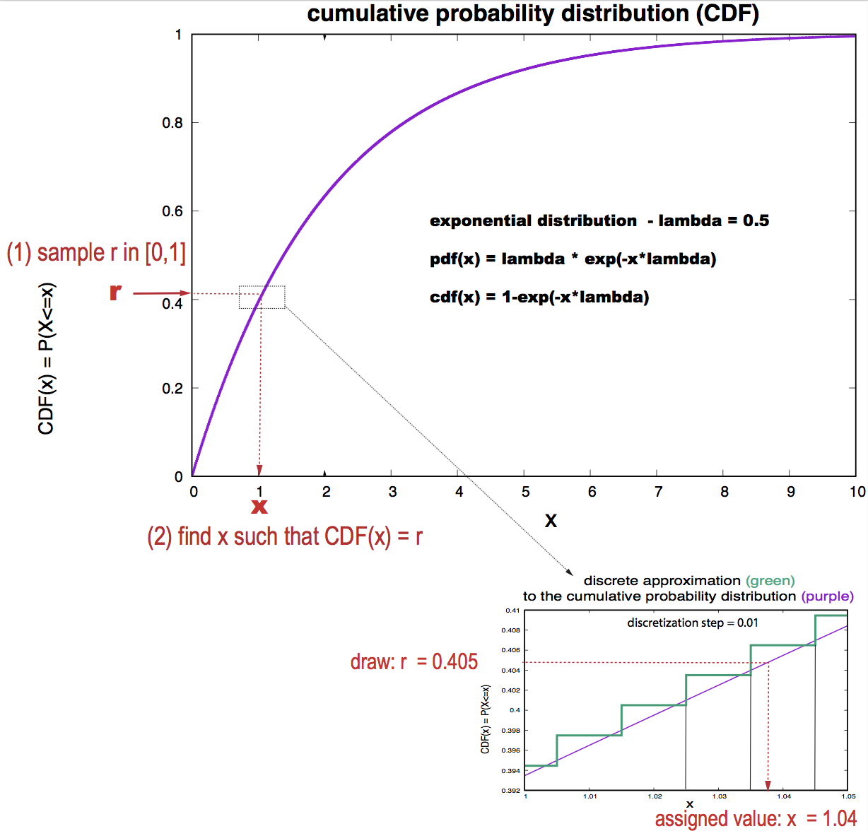
Figue 1. Sampling algorithm using only the rand() function. In purple, the exponential distribution for lambda = 0.5. In green, the discrete approximation using a window of size 0.01.
In general, for a probability density function (PDF) \(p(x)\), defined in a range \([x_{min},x_{max}]\), the cumulative distribution function (CDF) \(P(x)\) is given by
\begin{equation} P(x) = \int_{x_{\min}}^x p(y) dy \end{equation}
is a function that ranges over the interval [0,1], since it is a probability.
The simplest way is to construct the CDF numerically by discretizing the space \([x_{min},x_{max}]\) as,
\begin{equation} x_i = x_{min} + \Delta\,i \quad \mbox{in the range}\quad 1\leq i \leq N, \end{equation}
for some small interval value \(\Delta\), such that \(x_{max} = x_{min} + \Delta\,N\).
The discrete form of the CDF \(P\) is given by the \(N\) dimensional vector \begin{equation} \mbox{cdf}[i]\sim\sum_{j=1}^i p(x_{j})\, \Delta = \mbox{cdf}[i-1] + p(x_i)\,\Delta, \end{equation}
as described in the insert of Figure 1.
The sampling algorithm is:
1) Generate a random number \(r\) between 0 and 1
2) Find the index \(i\) such that
\begin{equation} \mbox{cdf}[i] \leq r < \mbox{cdf}[i+\Delta]. \end{equation}
Then the value sampled from the distribution is
\begin{equation} x = x_{min} + i\,\Delta. \end{equation}
That is, \(x\) is the highest value such that \(P(x) \leq r\). See Figure 1.